This document collects the supplementary materials for the white paper Equity
Analysis at a Large Scale: Using Small Area Estimation to Get the Most from the
CRDC School Arrest Data. It has four parts: exploratory analysis of the combined
three-year CRDC data, the data-construction and sample-restriction details,
model performance and diagnostics, and additional applied prediction-interval
examples. The headline tables and figures, and the national descriptive totals
by race and sex, are reported in the paper itself (white_paper.html); this
companion holds the supporting detail. Like the paper, every section reads the
published artifacts via crdc_path() and renders standalone.
Part 1 — Exploratory Data Analysis
This part explores the combined three-year CRDC data (2015-16, 2017-18, 2021-22). Counts and rates here are pooled across all three waves unless stated otherwise, and so differ from the single-wave 2021-22 figures in the paper.
Basic Data Structure
Data dimensions: 6762624 rows, 23 columns

'data.frame':   6762624 obs. of  23 variables:
 $ LEA_STATE            : chr  "AL" "AL" "AL" "AL" ...
 $ LEAID                : chr  "0100005" "0100005" "0100005" "0100005" ...
 $ SCHID                : int  870 870 870 870 870 870 870 870 870 870 ...
 $ SCH_NAME             : chr  "Albertville Middle School" "Albertville Middle School" "Albertville Middle School" "Albertville Middle School" ...
 $ COMBOKEY             : chr  "010000500870" "010000500870" "010000500870" "010000500870" ...
 $ JJ                   : chr  "No" "No" "No" "No" ...
 $ RACE                 : chr  "AM" "AM" "AS" "AS" ...
 $ SEX                  : chr  "F" "M" "F" "M" ...
 $ ARRESTS              : num  0 0 0 0 0 0 0 0 0 0 ...
 $ REFERRALS            : num  0 0 0 0 0 0 0 0 0 0 ...
 $ total_arrests        : num  0 0 0 0 0 0 0 0 0 0 ...
 $ total_referrals      : num  0 0 0 0 0 0 0 0 0 0 ...
 $ stu_enroll           : num  1 3 2 1 19 17 247 238 1 0 ...
 $ arrest_rate          : num  0 0 0 0 0 0 0 0 0 0 ...
 $ referral_rate        : num  0 0 0 0 0 0 0 0 0 0 ...
 $ YEAR                 : chr  "21-22" "21-22" "21-22" "21-22" ...
 $ total_enroll         : num  901 901 901 901 901 901 901 901 901 901 ...
 $ highest_grade_offered: num  8 8 8 8 8 8 8 8 8 8 ...
 $ lowest_grade_offered : num  7 7 7 7 7 7 7 7 7 7 ...
 $ latitude             : num  34.3 34.3 34.3 34.3 34.3 ...
 $ longitude            : num  -86.2 -86.2 -86.2 -86.2 -86.2 ...
 $ enrollment           : num  920 920 920 920 920 920 920 920 920 920 ...
 $ LEA_NAME             : chr  "Albertville City" "Albertville City" "Albertville City" "Albertville City" ...
| LEA_STATE | LEAID | SCHID | SCH_NAME | COMBOKEY | JJ | RACE | SEX | ARRESTS | REFERRALS | total_arrests | total_referrals | stu_enroll | arrest_rate | referral_rate | YEAR | total_enroll | highest_grade_offered | lowest_grade_offered | latitude | longitude | enrollment | LEA_NAME |
|---|---|---|---|---|---|---|---|---|---|---|---|---|---|---|---|---|---|---|---|---|---|---|
| AL | 0100005 | 870 | Albertville Middle School | 010000500870 | No | AM | F | 0 | 0 | 0 | 0 | 1 | 0 | 0 | 21-22 | 901 | 8 | 7 | 34.2602 | -86.2062 | 920 | Albertville City |
| AL | 0100005 | 870 | Albertville Middle School | 010000500870 | No | AM | M | 0 | 0 | 0 | 0 | 3 | 0 | 0 | 21-22 | 901 | 8 | 7 | 34.2602 | -86.2062 | 920 | Albertville City |
| AL | 0100005 | 870 | Albertville Middle School | 010000500870 | No | AS | F | 0 | 0 | 0 | 0 | 2 | 0 | 0 | 21-22 | 901 | 8 | 7 | 34.2602 | -86.2062 | 920 | Albertville City |
| AL | 0100005 | 870 | Albertville Middle School | 010000500870 | No | AS | M | 0 | 0 | 0 | 0 | 1 | 0 | 0 | 21-22 | 901 | 8 | 7 | 34.2602 | -86.2062 | 920 | Albertville City |
| AL | 0100005 | 870 | Albertville Middle School | 010000500870 | No | BL | F | 0 | 0 | 0 | 0 | 19 | 0 | 0 | 21-22 | 901 | 8 | 7 | 34.2602 | -86.2062 | 920 | Albertville City |
| AL | 0100005 | 870 | Albertville Middle School | 010000500870 | No | BL | M | 0 | 0 | 0 | 0 | 17 | 0 | 0 | 21-22 | 901 | 8 | 7 | 34.2602 | -86.2062 | 920 | Albertville City |
Table 1: First six rows of the combined CRDC analysis dataset
Summary Statistics by Year
| YEAR | n_observations | n_schools | n_districts | mean_enrollment | mean_arrests | mean_referrals |
|---|---|---|---|---|---|---|
| 15-16 | 2223792 | 92658 | 16648 | 88.27 | 0.11 | 0.41 |
| 17-18 | 2252736 | 93864 | 16642 | 87.64 | 0.09 | 0.38 |
| 21-22 | 2286096 | 95254 | 17624 | 83.43 | 0.06 | 0.36 |
Table 2: Observation counts and mean enrollment, arrests, and referrals by CRDC collection year
Summary Plot of Trends
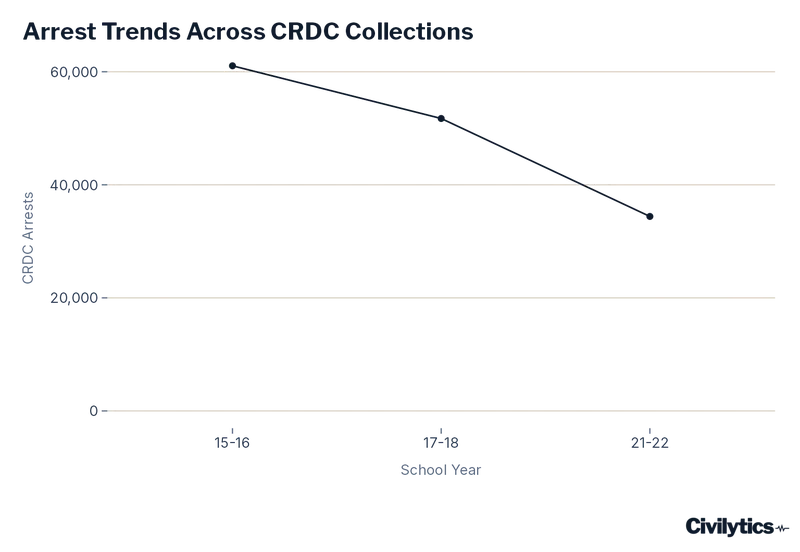
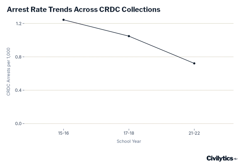
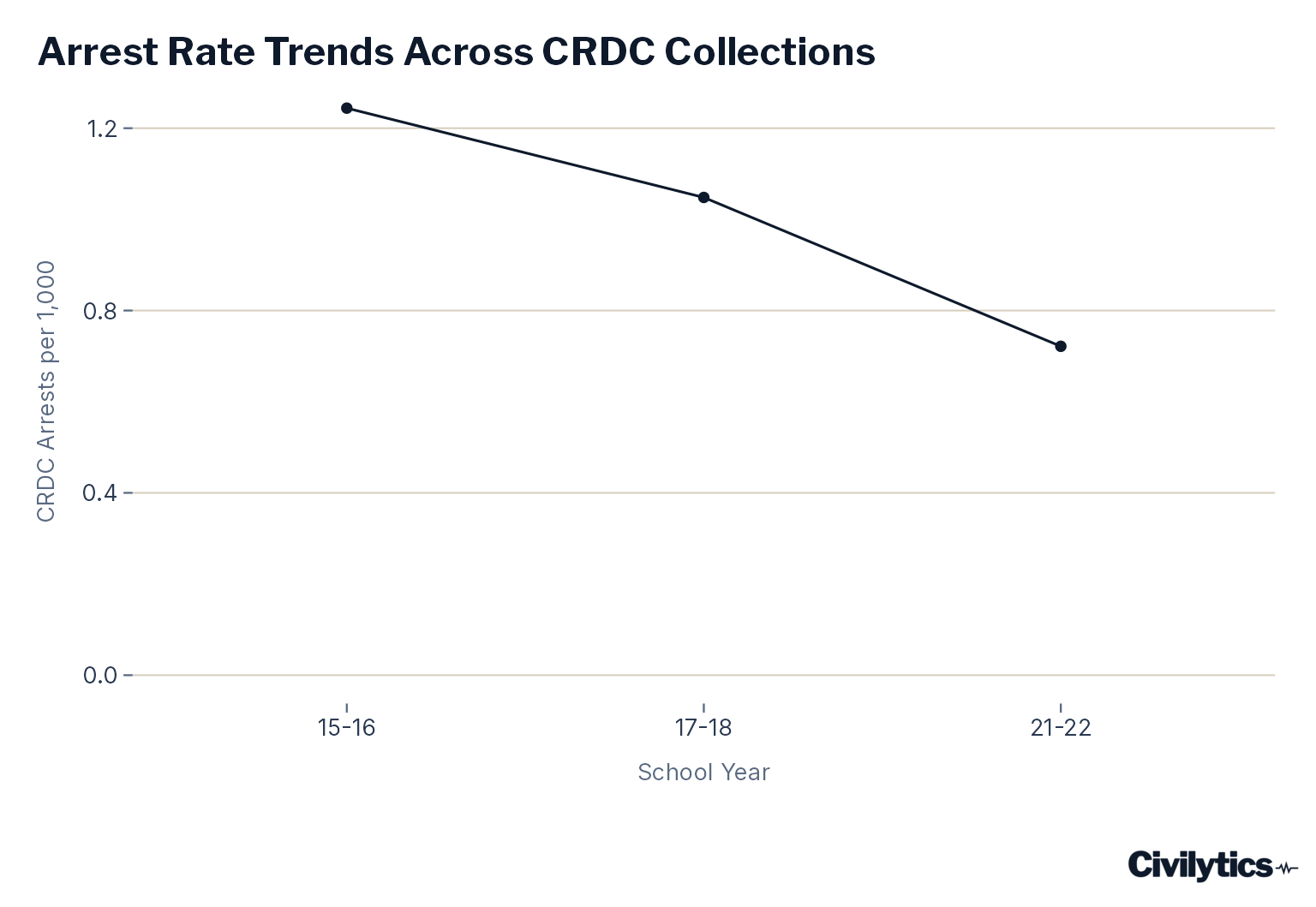
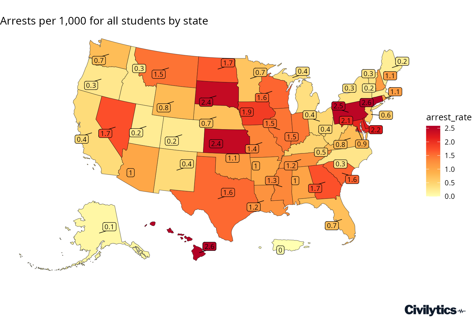
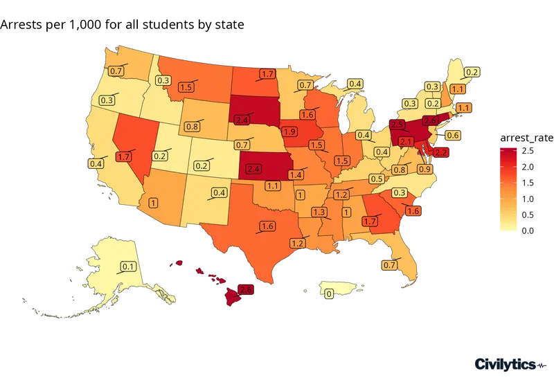
State Variation Summing over 3 years
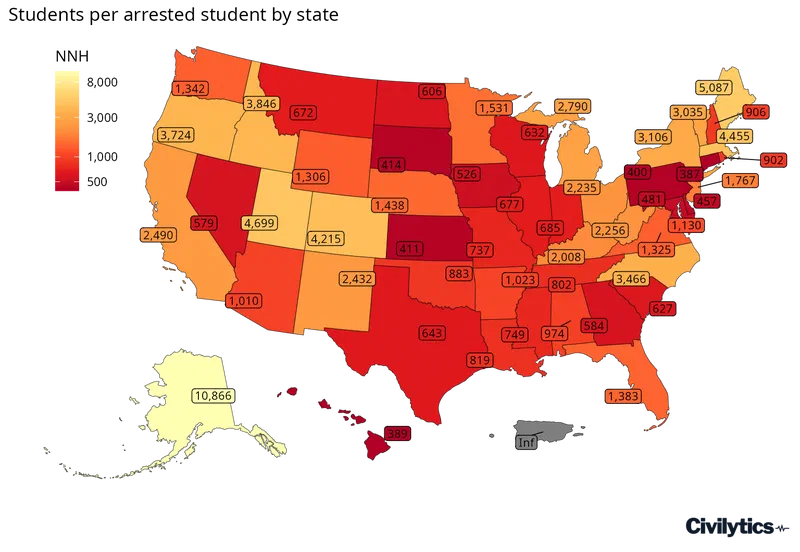
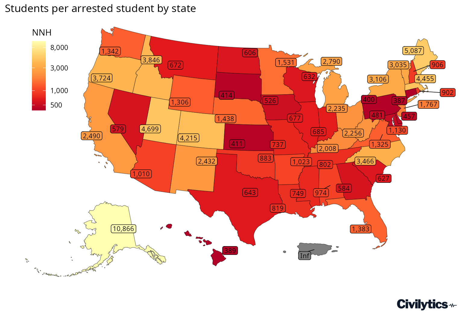
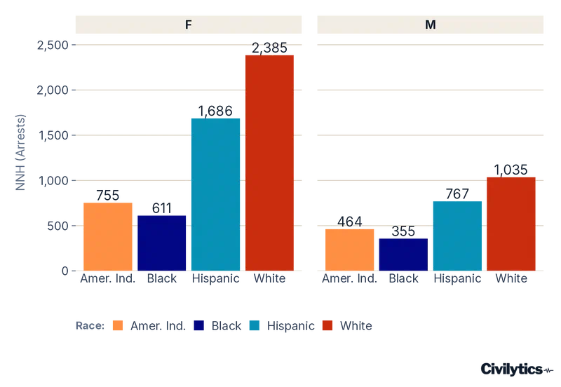
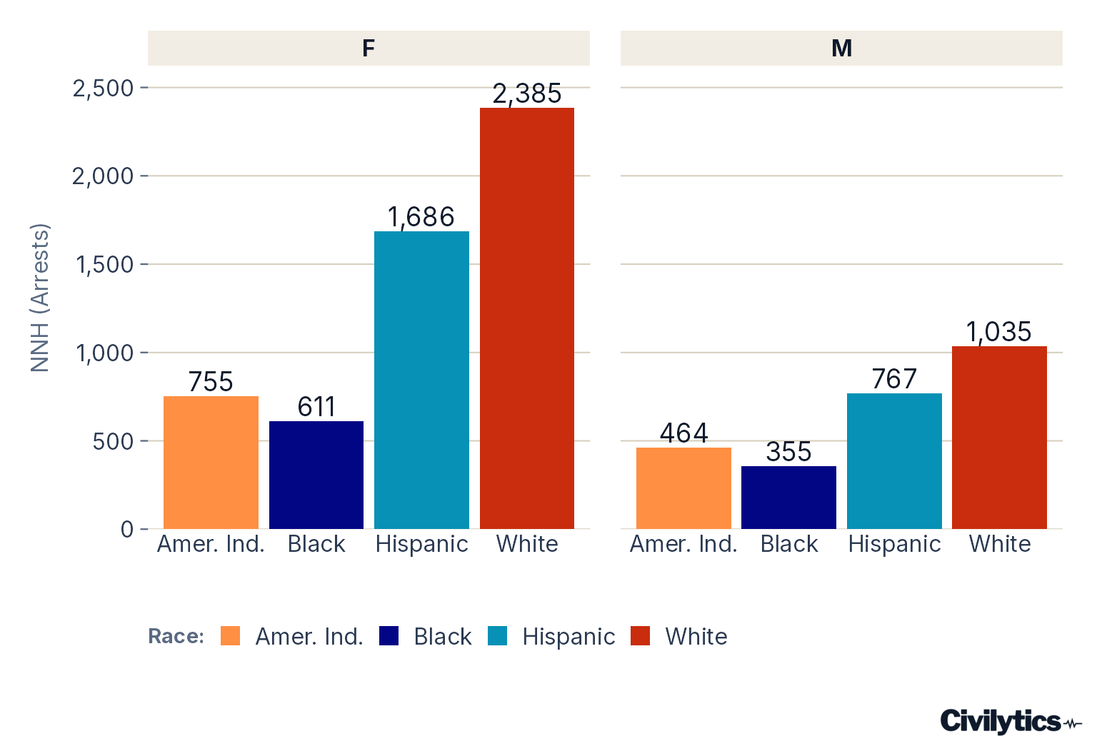
Race and Sex Distribution
These counts and rates are pooled across all three CRDC waves (2015-16,
2017-18, 2021-22) and are shown here as number-needed-to-harm (NNH, students
per arrested student). They therefore differ from the single-wave 2021-22
totals and per-1,000 rates reported in white_paper.qmd; they are not the same
figures and should not be read as such.
| RACE | SEX | n_observations | total_enrollment | total_arrests | total_referrals | arrest_rate |
|---|---|---|---|---|---|---|
| WH | M | 281776 | 36086936 | 34858 | 173588 | 0.966 |
| BL | M | 281776 | 11160417 | 31449 | 120242 | 2.818 |
| HI | M | 281776 | 20045187 | 26127 | 110494 | 1.303 |
| BL | F | 281776 | 10716558 | 17539 | 65871 | 1.637 |
| WH | F | 281776 | 33822299 | 14184 | 72807 | 0.419 |
| HI | F | 281776 | 19115302 | 11341 | 52161 | 0.593 |
| TR | M | 281776 | 2993936 | 4187 | 20757 | 1.398 |
| TR | F | 281776 | 2896769 | 2171 | 10713 | 0.749 |
| AM | M | 281776 | 753932 | 1626 | 7630 | 2.157 |
| AS | M | 281776 | 3694856 | 1255 | 7404 | 0.340 |
| AM | F | 281776 | 720578 | 955 | 4471 | 1.325 |
| HP | M | 281776 | 297420 | 724 | 2052 | 2.434 |
| AS | F | 281776 | 3527728 | 430 | 2674 | 0.122 |
| HP | F | 281776 | 280560 | 336 | 979 | 1.198 |
Table 3: Arrest counts, enrollment, and arrest rates by race and sex, pooled across all three CRDC waves
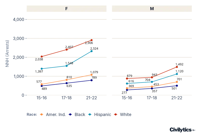
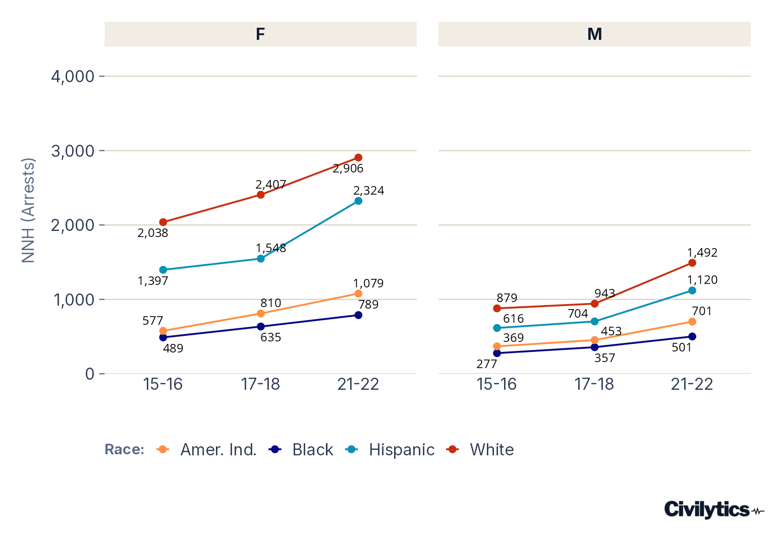
Trends by group
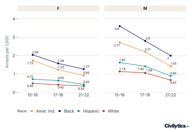
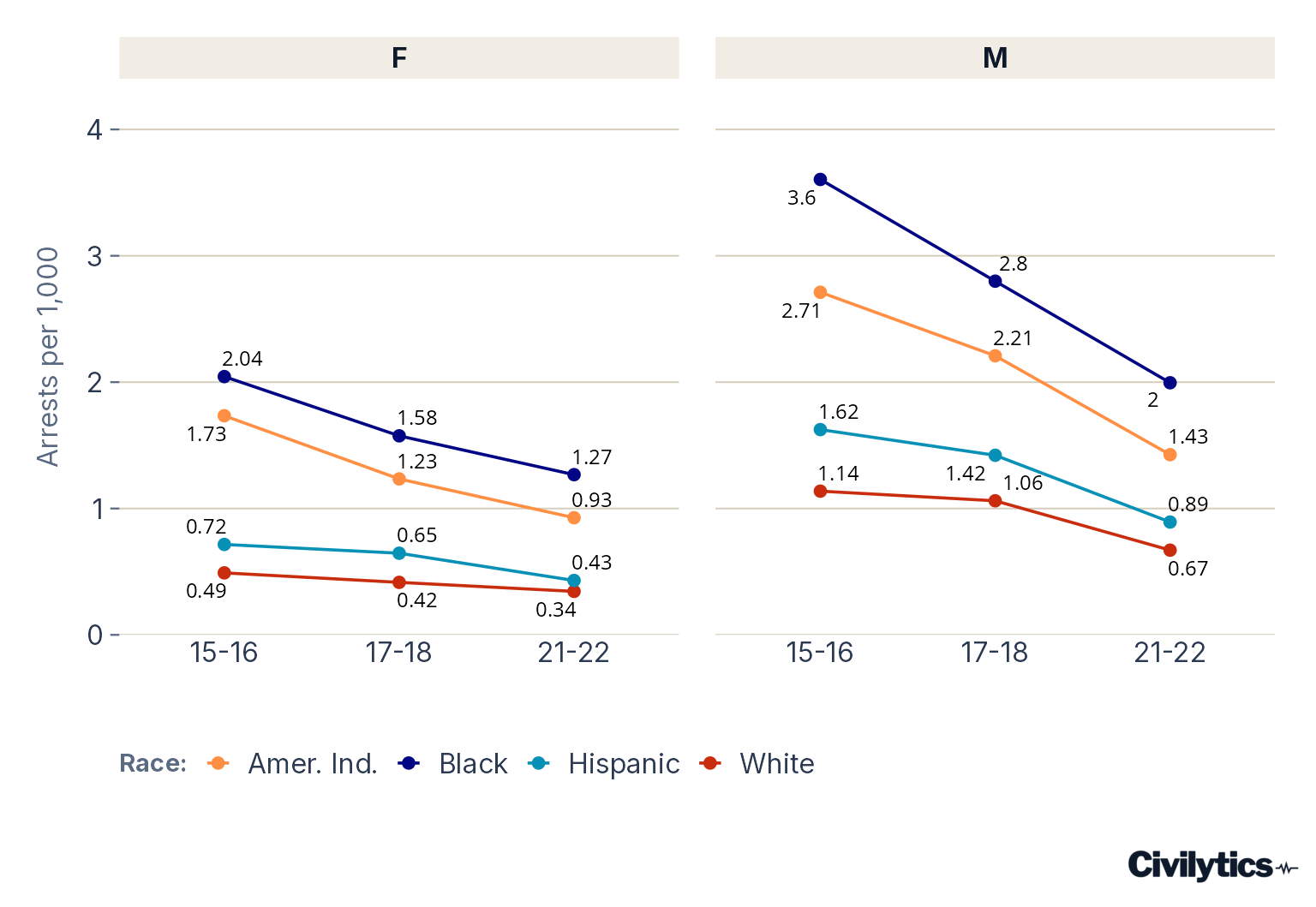
State Trends
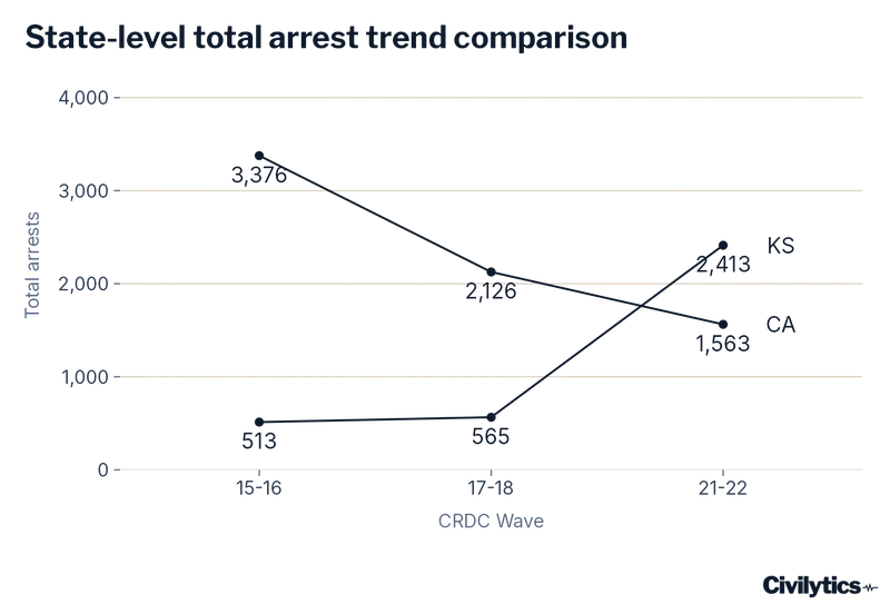
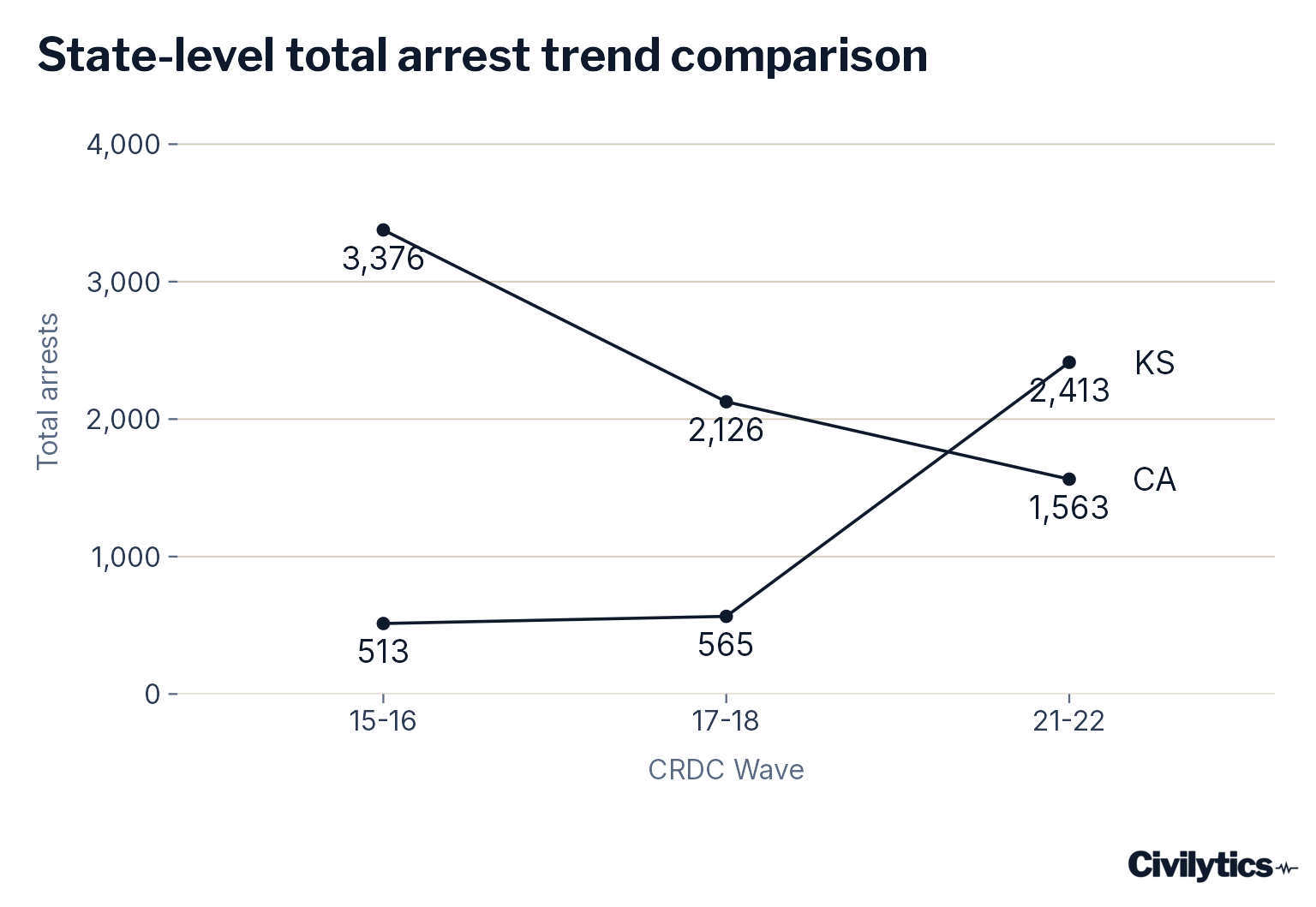
LEA Comparison
If we aggregate to the LEA level, what patterns do we see?
         1          2          3
0.09864719 0.04783550 0.85351732

[1] 18480

[1] 0.01894883 0.01585647 0.96519470
Rankings over time
| State | LEA Name | Enrollment (21-22) | Arrests (21-22) | Arrest Rate (21-22) | Arrests (17-18) | Arrests (15-16) |
|---|---|---|---|---|---|---|
| IL | DeKalb CUSD 428 | 6089 | 2197 | 360.81 | 8 | 0 |
| KS | Derby | 6410 | 2092 | 326.37 | 112 | 0 |
| FL | PINELLAS | 92094 | 601 | 6.53 | 498 | 0 |
| TX | PASADENA ISD | 47049 | 456 | 9.69 | 389 | 426 |
| GA | Cobb County | 106062 | 416 | 3.92 | 177 | 315 |
| TX | ECTOR COUNTY ISD | 30043 | 405 | 13.48 | 402 | 107 |
| MD | Anne Arundel County Public Schools | 83544 | 386 | 4.62 | 255 | 0 |
| GA | Richmond County | 28191 | 361 | 12.81 | 25 | 10 |
| PA | Chambersburg Area SD | 8901 | 274 | 30.78 | 80 | 103 |
| GA | Gwinnett County | 178437 | 268 | 1.50 | 518 | 892 |
| FL | BROWARD | 250480 | 258 | 1.03 | 13 | 140 |
| TX | SOCORRO ISD | 44440 | 258 | 5.81 | 0 | 0 |
| LA | Jefferson Parish | 45153 | 242 | 5.36 | 188 | 379 |
| SD | Rapid City Area School District 51-4 | 12815 | 241 | 18.81 | 194 | 176 |
| GA | Bibb County | 20479 | 222 | 10.84 | 215 | 140 |
| FL | MIAMI-DADE | 320607 | 221 | 0.69 | 128 | 203 |
| LA | Terrebonne Parish | 14575 | 217 | 14.89 | 6 | 14 |
| CT | Waterbury School District | 17681 | 209 | 11.82 | 248 | 212 |
| CA | San Diego Unified | 96295 | 208 | 2.16 | 365 | 228 |
| TX | GARLAND ISD | 51271 | 201 | 3.92 | 209 | 45 |
Table 4: The 20 districts with the most total arrests in 2021-22, with enrollment, arrest rate, and prior-wave arrest counts
Rankings of arrest rates
| State | LEA Name | Arrest Rate (21-22) | Arrest Rate (17-18) | Arrest Rate (15-16) | Enrollment (21-22) | Arrests (21-22) | Arrests (17-18) | Arrests (15-16) |
|---|---|---|---|---|---|---|---|---|
| MO | PEMISCOT CO. SPEC. SCH. DIST. | 442.9 | NA | 0.0 | 219 | 97 | NA | 0 |
| IL | DeKalb CUSD 428 | 360.8 | 1.2 | 0.0 | 6089 | 2197 | 8 | 0 |
| KS | Derby | 326.4 | 15.9 | 0.0 | 6410 | 2092 | 112 | 0 |
| AZ | Yuma Private Industry Council Inc. (4509) | 137.9 | 36.4 | 0.0 | 116 | 16 | 4 | 0 |
| WA | Mabton School District | 134.2 | 0.0 | 0.0 | 678 | 91 | 0 | 0 |
| MN | MN VALLEY EDUCATION DISTRICT | 115.4 | 0.0 | 0.0 | 52 | 6 | 0 | 0 |
| PA | Dr Robert Ketterer CS Inc | 114.5 | 6.0 | 0.0 | 166 | 19 | 1 | 0 |
| IL | Kaskaskia Spec Educ District | 95.2 | 33.3 | 0.0 | 105 | 10 | 4 | 0 |
| IL | Four Rivers Spec Educ Dist | 87.0 | 576.9 | 287.9 | 92 | 8 | 30 | 19 |
| NM | ZUNI PUBLIC SCHOOLS | 58.0 | 19.4 | 7.0 | 1155 | 67 | 24 | 9 |
| IL | Pekin CSD 303 | 54.0 | 26.9 | 20.0 | 1814 | 98 | 49 | 40 |
| IL | La Salle-Peru Twp HSD 120 | 50.4 | 17.2 | 36.3 | 1310 | 66 | 21 | 45 |
| MT | Wolf Point H S | 46.0 | 0.0 | 0.0 | 239 | 11 | 0 | 0 |
| WY | Carbon County School District #1 | 42.9 | 0.0 | 1.1 | 1585 | 68 | 0 | 2 |
| AZ | Mingus Union High School District (4488) | 42.0 | 40.6 | 38.1 | 1356 | 57 | 50 | 47 |
| MN | EAST RANGE ACADEMY OF TECH-SCIENCE | 37.7 | 0.0 | 0.0 | 106 | 4 | 0 | 0 |
| TX | SHEPHERD ISD | 37.1 | 0.0 | 2.1 | 1912 | 71 | 0 | 4 |
| IL | Ogle Co Education Cooperative | 35.4 | 62.5 | 189.2 | 113 | 4 | 2 | 7 |
| PA | McGuffey SD | 34.1 | 0.0 | 6.5 | 1552 | 53 | 0 | 11 |
| WI | New Holstein School District | 34.1 | 9.3 | 1.8 | 938 | 32 | 10 | 2 |
Table 5: The 20 districts with the highest arrest rate in 2021-22, with enrollment, arrest counts, and prior-wave arrest rates
Part 2 — Data Construction & Sample Restrictions
This part documents how the analytic sample is built from the raw CRDC and the
magnitude of each restriction the paper describes. The national descriptive
totals and rates by race and sex are reported in the paper (white_paper.html).
Sample Continuity Analysis for CRDC Waves
Look at how many LEAs are in multiple years of data and how many LEAs drop out of the data when we add successive waves of the data.
**** Distinct Matches ****
**** Match Summary ****
X in Y
Of the 17604 X values, 16203 (92%) were matched.
********************************************
Y in X
Of the 17704 Y values, 16203 (92%) were matched.
******************************************

**** Distinct Matches ****
**** Match Summary ****
X in Y
Of the 17337 X values, 15877 (92%) were matched.
********************************************
Y in X
Of the 16203 Y values, 15877 (98%) were matched.
******************************************
District Concentration Analysis
For this analysis we look at the most recent CRDC wave.
District Size Categories
Expected vs Observed Arrests
| popcut | dists | dists_w_arrests | expec_distw_arrests | dist_w_arrest_per | expect_w_arrest_per |
|---|---|---|---|---|---|
| 0-999 | 10323 | 336 | 448.6 | 3.3% | 4.3% |
| 1,000-9,999 | 6515 | 1210 | 3418.7 | 18.6% | 52.5% |
| 10,000-19,999 | 490 | 263 | 489.2 | 53.7% | 99.8% |
| 20,000+ | 376 | 251 | 376.0 | 66.8% | 100.0% |
Table 6: Observed and expected districts with at least one arrest, by district size
Concentration Visualization
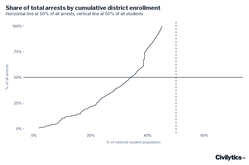
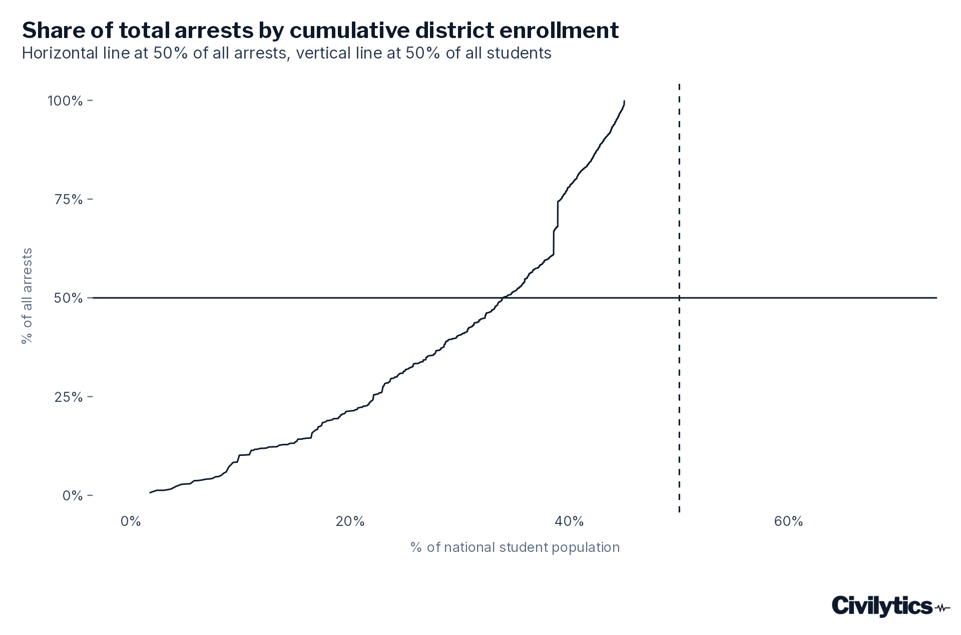
This visualization shows the relative concentration of arrests compared in LEAs compared to the concentration of population in LEAs.
Enrollment by Arrest Status
| has_arrest | enrollment | enrollment_per |
|---|---|---|
| Arrests | 21860332 | 0.4498336 |
| No arrests | 26736157 | 0.5501664 |
Table 7: Share of national student enrollment in districts with and without any reported arrest
Sample Restriction Impact
Here we tabulate the figures about sample restrictions in the paper.
Section 504 Data
| SCH_DISCWDIS_REF_504_M | SCH_DISCWDIS_REF_504_F | SCH_DISCWDIS_ARR_504_M | SCH_DISCWDIS_ARR_504_F |
|---|---|---|---|
| 7863 | 3239 | 1252 | 533 |
Table 8: Summary of Section 504 disability status among law enforcement referrals
Missing Data Patterns
Law enforcement referral missingness data.
  FALSE    TRUE
5303388  185172


     FALSE       TRUE
0.96626219 0.03373781
Section 504 Enrollment
| SCH_ENR_504_M | SCH_ENR_504_F |
|---|---|
| 978195 | 713670 |
Table 9: Total Section 504-eligible student enrollment
Grade Level Restrictions
This reports the impact of restricting the analysis to schools that offer a grade 7 or above.
| hs | enrollment | arrests | referrals |
|---|---|---|---|
| No | 19785585 | 1453 | 13760 |
| Yes | 28625386 | 32950 | 192678 |
| NA | 0 | 0 | 4 |
Table 10: Enrollment, arrests, and referrals by whether a school offers grade 7 or above
CCD Matching
By matching to CCD data we further restrict the CRDC universe. This analysis shows the impact of that.
**** Distinct Matches ****
**** Match Summary ****
X in Y
Of the 98010 X values, 95254 (97%) were matched.
********************************************
Y in X
Of the 102130 Y values, 95254 (93%) were matched.
******************************************
| in_ccd | enrollment | arrests | referrals |
|---|---|---|---|
| No | 914380 | 443 | 2911 |
| Yes | 47682109 | 34403 | 206442 |
Table 11: Enrollment, arrests, and referrals by whether a school matched to CCD geographic data
            used   (Mb) gc trigger   (Mb)  max used   (Mb)
Ncells   4395634  234.8   15070707  804.9  29434972 1572.0
Vcells 219785437 1676.9  441836648 3371.0 454062917 3464.3
Enrollment Thresholds
We restrict the sample by enrollment size, and this reports the impact of that restriction.
| filtered_out | dists | enrollment | arrests | referrals |
|---|---|---|---|---|
| No | 16281 | 28636189 | 32914 | 192604 |
| Yes | 308 | 4693 | 1 | 19 |
Table 12: Districts, enrollment, arrests, and referrals by whether a district falls below the minimum-enrollment threshold
Censored or truncated enrollment data
Here we report the impact of suppressed records on enrollment.
[1] 0.01887051
Part 3 — Model Performance & Diagnostics
Model Predictions and Performance
Now we calculate the performance results comparing the models to non-model methods for computing arrest rates.
Observed Data Preparation
Performance Metrics
This code calculates our performance metrics on the arrest rate scale, translating it from the arrest scale.
Full-sample model performance
The full-sample summary of coverage, precision, “% equal or better” intervals,
and median % narrowed across all ten models is Table 3 in white_paper.qmd,
computed there from this same observed-vs-modeled join. It is not duplicated
here. The diagnostic cross-tabulations that are unique to this document follow.
Model Performance Diagnostics
Comparing models to non-modeled intervals
                 improved_precision
narrower_interval       0       1
                0   12475    4738
                1     936 1048881

                 improved_precision
narrower_interval       0       1
                0   12661    4552
                1 1049737      80
Looking at constant models
Some fitted values are constants with no variation. We want to look at these cases separately.
| fitted_constant | Freq |
|---|---|
| 0 | 0.6706456 |
| 1 | 0.3293544 |
Table 13: Share of model fitted values that are constant across posterior draws
When we exclude constant prediction results and see how models perform to non-modeled intervals.
        higher_precsion
narrower      0      1
       0  12475   4738
       1    936 697450
Non-Constant Models
Now we look in more depth at results from observations without constant predicted values.
| model_id | YEAR | count | obsv_precision | fit_precision | covered | per_covered | per_improved_cv | per_narrower | per_improved_pre |
|---|---|---|---|---|---|---|---|---|---|
| stratified_m1_mod | 21-22 | 91818 | 0.4494722 | 2.867553 | 91818 | 1.0000000 | 0.0000000 | 0.9846980 | 0.9820950 |
| stratified_m2_mod | 21-22 | 59387 | 0.6943254 | 7.998808 | 59364 | 0.9996127 | 0.0000000 | 0.9719804 | 0.9720478 |
| stratified_m3_mod | 21-22 | 92861 | 0.4444339 | 2.786696 | 91539 | 0.9857637 | 0.0092612 | 0.9719904 | 0.9811008 |
| stratified_m4_mod | 21-22 | 68448 | 0.6026573 | 6.319210 | 67775 | 0.9901677 | 0.0064721 | 0.9735273 | 0.9803793 |
| stratified_m5_mod | 21-22 | 67652 | 0.6096470 | 6.723667 | 66985 | 0.9901407 | 0.0065187 | 0.9730385 | 0.9800302 |
| unified_m1_mod | 21-22 | 75349 | 0.5474304 | 12.117737 | 75060 | 0.9961645 | 0.0032515 | 0.9830257 | 0.9859321 |
| unified_m2_mod | 21-22 | 56660 | 0.7276874 | 12.615769 | 56553 | 0.9981115 | 0.0018885 | 0.9817155 | 0.9833392 |
| unified_m3_mod | 21-22 | 76981 | 0.5357239 | 8.274921 | 75218 | 0.9770982 | 0.0153544 | 0.9690313 | 0.9800340 |
| unified_m4_mod | 21-22 | 63171 | 0.6527878 | 8.688558 | 62286 | 0.9859904 | 0.0106378 | 0.9746878 | 0.9832835 |
| unified_m5_mod | 21-22 | 63272 | 0.6517935 | 8.714473 | 62394 | 0.9861234 | 0.0107789 | 0.9745701 | 0.9832311 |
Table 14: Model performance metrics by model and year, excluding constant predictions
Non-zero-arrest model performance
Model performance restricted to district-student groups with at least one
observed arrest is Table 4 in white_paper.qmd. It is not duplicated here.
Subgroup Analysis
Define Subgroups
Create largest 100 districts
The “most total arrests” and “largest-enrollment with zero arrests” district
subsets are analysed canonically in white_paper.qmd (Tables 5 and 6), so only
the largest-enrollment-by-any-arrest subset (big100) is built here.
Large Districts Performance
Look at how models perform on the 100 largest districts by student enrollment
| model_id | YEAR | count | obsv_precision | fit_precision | obsv_interval_med | fit_interval_med | interval_delta | improved_precision | improved_interval | covered | per_covered | per_narrower | per_improved_pre |
|---|---|---|---|---|---|---|---|---|---|---|---|---|---|
| stratified_m1_mod | 21-22 | 800 | 35.73036 | 94.65824 | 1.941881 | 1.0076510 | 0.3333333 | 588 | 600 | 800 | 1.00000 | 0.75000 | 0.73500 |
| stratified_m2_mod | 21-22 | 800 | 35.73036 | 75.39027 | 1.941881 | 0.7125790 | 0.3333333 | 587 | 575 | 800 | 1.00000 | 0.71875 | 0.73375 |
| stratified_m3_mod | 21-22 | 800 | 35.73036 | 44.36768 | 1.941881 | 1.0686044 | 0.3333333 | 561 | 540 | 609 | 0.76125 | 0.67500 | 0.70125 |
| stratified_m4_mod | 21-22 | 800 | 35.73036 | 51.76967 | 1.941881 | 0.8940119 | 0.3333333 | 607 | 579 | 661 | 0.82625 | 0.72375 | 0.75875 |
| stratified_m5_mod | 21-22 | 800 | 35.73036 | 51.45227 | 1.941881 | 0.8845061 | 0.3333333 | 600 | 581 | 659 | 0.82375 | 0.72625 | 0.75000 |
| unified_m1_mod | 21-22 | 800 | 35.73036 | 478.79275 | 1.941881 | 0.6574109 | 0.5308079 | 662 | 647 | 762 | 0.95250 | 0.80875 | 0.82750 |
| unified_m2_mod | 21-22 | 800 | 35.73036 | 262.61855 | 1.941881 | 0.5220347 | 0.5303936 | 680 | 663 | 785 | 0.98125 | 0.82875 | 0.85000 |
| unified_m3_mod | 21-22 | 800 | 35.73036 | 82.79272 | 1.941881 | 1.4027286 | 0.3333333 | 564 | 535 | 592 | 0.74000 | 0.66875 | 0.70500 |
| unified_m4_mod | 21-22 | 800 | 35.73036 | 65.55298 | 1.941881 | 0.8779633 | 0.3333333 | 618 | 588 | 646 | 0.80750 | 0.73500 | 0.77250 |
| unified_m5_mod | 21-22 | 800 | 35.73036 | 64.59302 | 1.941881 | 0.8829440 | 0.3333333 | 618 | 581 | 648 | 0.81000 | 0.72625 | 0.77250 |
Table 15: Model performance for the 100 largest-enrollment districts by model and year
High-arrest and zero-arrest district performance
Model performance for the 100 districts with the most total arrests is Table
5, and the expected-vs-observed arrests for the 100 largest-enrollment
districts that reported zero arrests is Table 6 — both computed reproducibly
in white_paper.qmd. They are not duplicated here.
Model Computation Statistics
Here we compute the model statistics.
Unified Models
| Model | ndraws | chains | threads | thin | leas | parameters | worst_rhat | min_bulk_ess | mean_bulk_ess | runtime_minutes | data_rows |
|---|---|---|---|---|---|---|---|---|---|---|---|
| Unified (m1) | 5250 | 3 | 4 | 1 | 16279 | 16339 | 1.010254 | 263.7597 | 742.7275 | 26.88767 | 106703 |
| Unified (m2) | 7000 | 4 | 4 | 1 | 16279 | 16340 | 1.003690 | 871.1463 | 1570.4588 | 62.64267 | 106703 |
| Unified (m3) | 7000 | 4 | 4 | 1 | 17039 | 17101 | 1.011419 | 491.7582 | 3157.1301 | 217.06500 | 307468 |
| Unified (m4) | 4000 | 4 | 4 | 2 | 17039 | 17102 | 1.002415 | 1024.7808 | 2423.7256 | 375.43000 | 307468 |
| Unified (m5) | 4000 | 4 | 4 | 2 | 17039 | 17103 | 1.005188 | 1103.0185 | 2431.2921 | 280.92667 | 307468 |
Table 16: Sampler configuration and convergence diagnostics for the unified models
Stratified Models
# A tibble: 0 × 5
# ℹ 5 variables: model_label <chr>, runtime <dbl>, parameters <dbl>, data_rows <int>, ndraws <dbl>
HMC Diagnostics
### Unified (m1)

Divergences:
Tree depth:
Energy:
### Unified (m2)

Divergences:
Tree depth:
Energy:
### Unified (m3)

Divergences:
Tree depth:
Energy:
### Unified (m4)

Divergences:
Tree depth:
Energy:
### Unified (m5)

Divergences:
Tree depth:
Energy:
State-Level Analysis
State Predictions
            used   (Mb) gc trigger   (Mb)  max used   (Mb)
Ncells   4662848  249.1   15070707  804.9  29434972 1572.0
Vcells 142568456 1087.8  425250724 3244.5 531563027 4055.6
State Observed Data
State Performance
| model_id | YEAR | count | meanCVP | meanfitCVP | obsv_precision | fit_precision | improved_cv | improved_precision | covered | per_covered | per_improved_cv | per_improved_pre |
|---|---|---|---|---|---|---|---|---|---|---|---|---|
| stratified_m1_mod | 21-22 | 408 | 32.23973 | 965.4790 | 192.4665 | 32026.77 | 0 | 398 | 78 | 0.1911765 | 0.0000000 | 0.9754902 |
| stratified_m2_mod | 21-22 | 408 | 32.23973 | 1161.2785 | 192.4665 | 33132.19 | 0 | 396 | 79 | 0.1936275 | 0.0000000 | 0.9705882 |
| stratified_m3_mod | 21-22 | 408 | 32.23973 | 814.9825 | 192.4665 | 17847.93 | 5 | 396 | 87 | 0.2132353 | 0.0122549 | 0.9705882 |
| stratified_m4_mod | 21-22 | 408 | 32.23973 | 1034.9360 | 192.4665 | 26962.45 | 5 | 392 | 85 | 0.2083333 | 0.0122549 | 0.9607843 |
| stratified_m5_mod | 21-22 | 408 | 32.23973 | 1059.1324 | 192.4665 | 26682.81 | 5 | 392 | 85 | 0.2083333 | 0.0122549 | 0.9607843 |
| unified_m1_mod | 21-22 | 408 | 32.23973 | 922.8268 | 192.4665 | 26953.97 | 0 | 398 | 85 | 0.2083333 | 0.0000000 | 0.9754902 |
| unified_m2_mod | 21-22 | 408 | 32.23973 | 1217.4136 | 192.4665 | Inf | NA | 401 | 82 | 0.2009804 | NA | 0.9828431 |
| unified_m3_mod | 21-22 | 408 | 32.23973 | 733.8663 | 192.4665 | 18771.01 | 6 | 395 | 90 | 0.2205882 | 0.0147059 | 0.9681373 |
| unified_m4_mod | 21-22 | 408 | 32.23973 | 1033.6301 | 192.4665 | Inf | NA | 392 | 85 | 0.2083333 | NA | 0.9607843 |
| unified_m5_mod | 21-22 | 408 | 32.23973 | 1037.4246 | 192.4665 | 22155.81 | 5 | 391 | 85 | 0.2083333 | 0.0122549 | 0.9583333 |
Table 18: State-level model performance metrics by model and year
Part 4 — Applied Examples
These are additional applied prediction-interval examples beyond the case studies in the paper: a cross-district comparison, a single-district temporal comparison, a small-groups demographic disparity, and a national overview.
Cross-district, temporal, and small-group comparisons
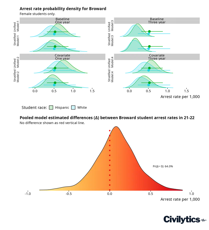
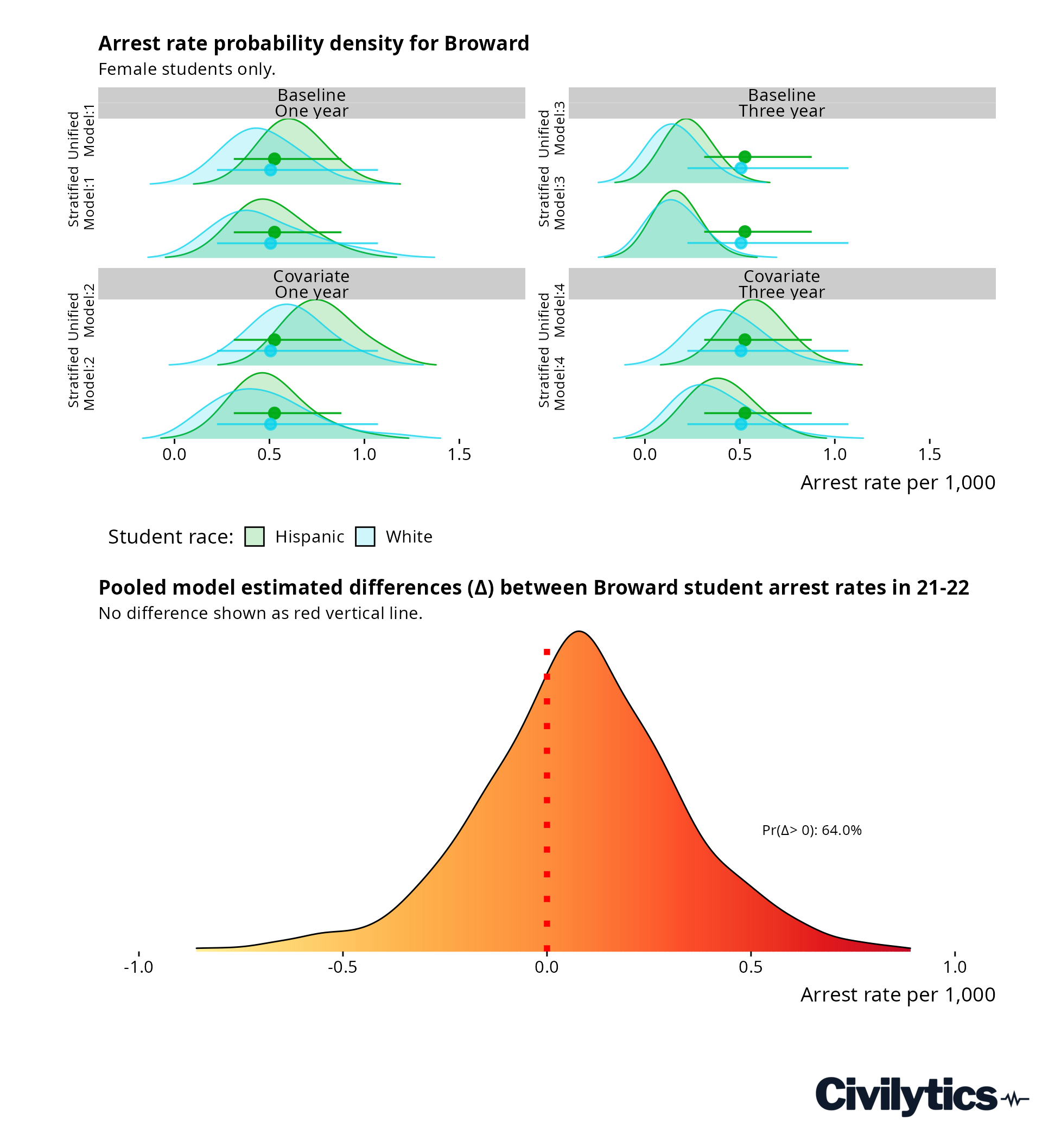
Compare Baltimore City to Baltimore County Baltimore City to itself last year Broward White Female to Hispanic female
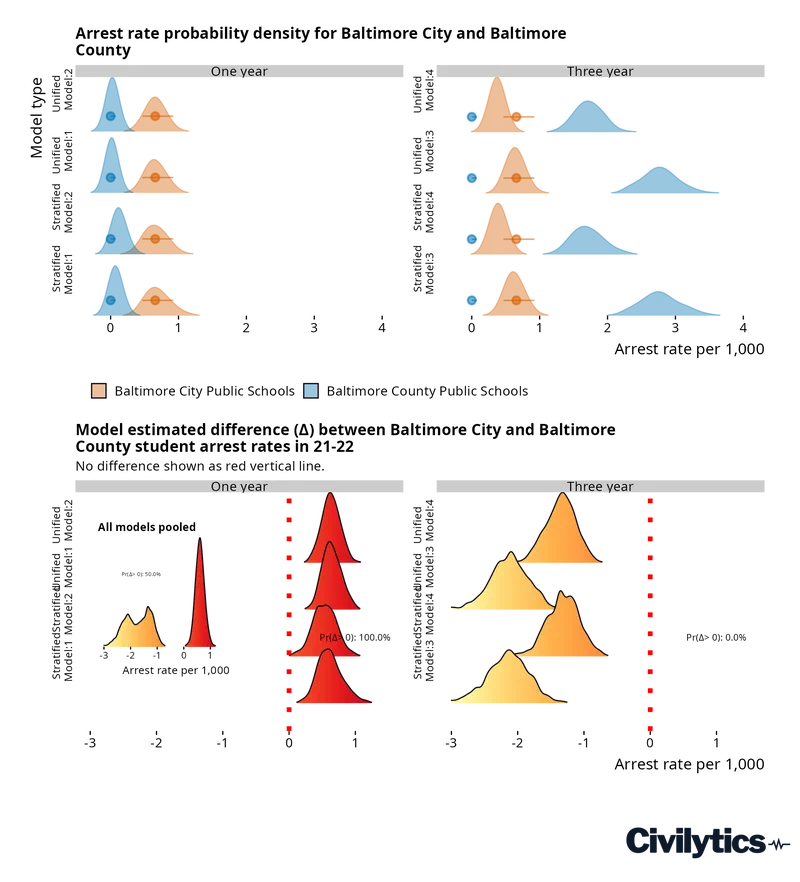
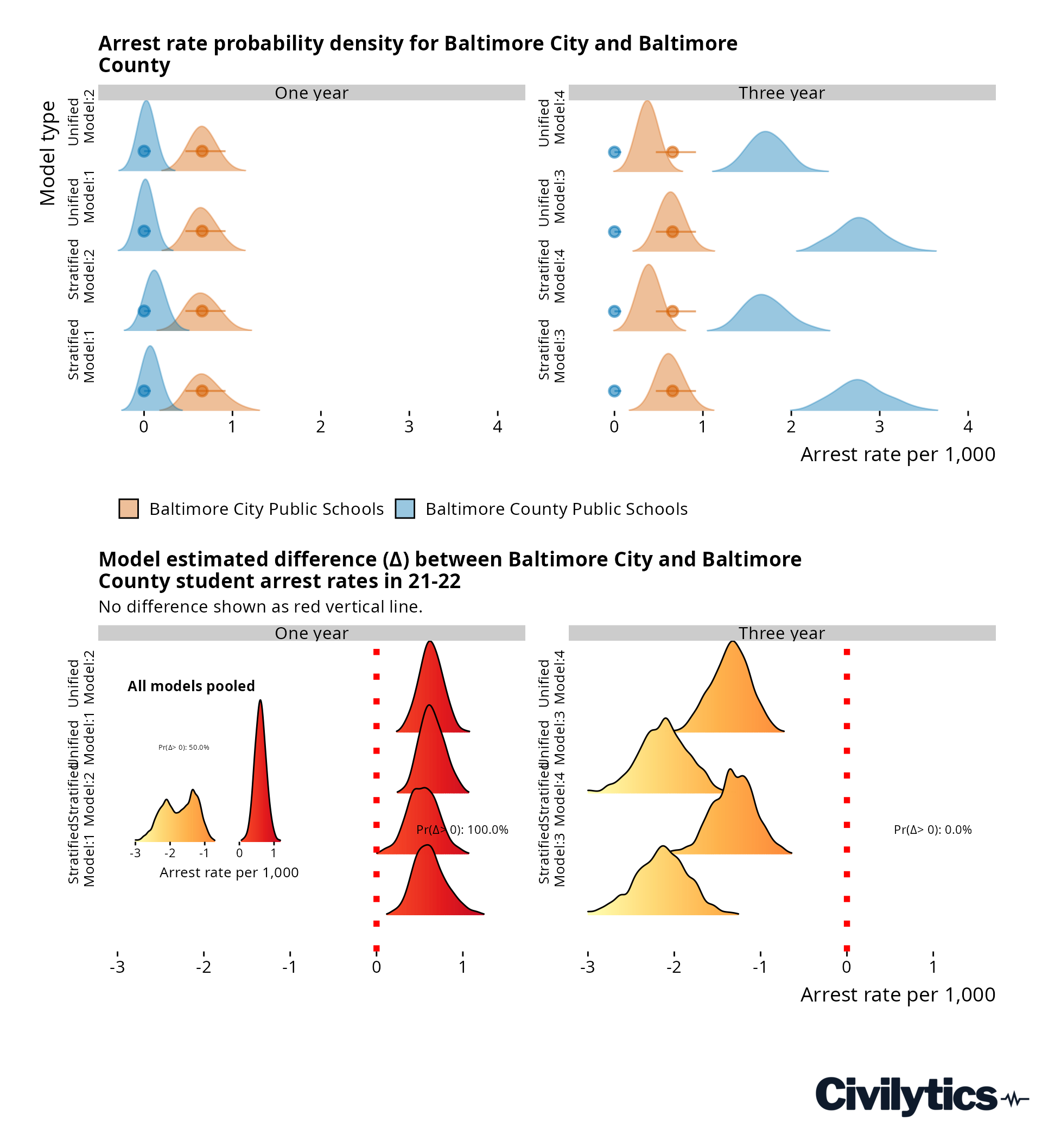
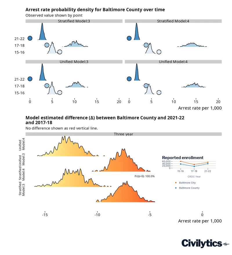
Here we apply the same approach as above but to compare arrest rates from two different school districts - Baltimore City Public Schools (orange) and Baltimore County Public Schools (blue). Here we see a curious pattern - if we look at our one year models, the frequentist interval and Bayesian intervals strongly agree that Baltimore City has a higher arrest rate than Baltimore County, with the most likely arrest rate in Baltimore County being 0. Covariates make little difference in these estimates.
The three year models have a very different picture - the Bayesian models see Baltimore County as having not just a higher arrest rate, but a much higher arrest rate than Baltimore City. The Baltimore City estimates are relatively unchanged, though covariates seem to shift the distribution slightly closer to 0 (unified and stratified models 4).
When we turn to our direct estimate of the differences, we see this pattern play out - the one year models are 100% certain in all specifications that Baltimore City has a higher arrest rate than Baltimore County, and that difference is most likely narrowly between just greater than 0 and 1. In contract, the 3 year models are equally sure that Baltimore City has no chance of a higher arrest rate than Baltimore County, and in fact, that it is most likely that Baltimore County’s arrest rate is 1-2 arrests per 1,000 greater than Baltimore City. When we pool all of our models together, we are left with a 50% chance one of the Baltimore’s has a greater arrest rate than the other (inset, bottom left).
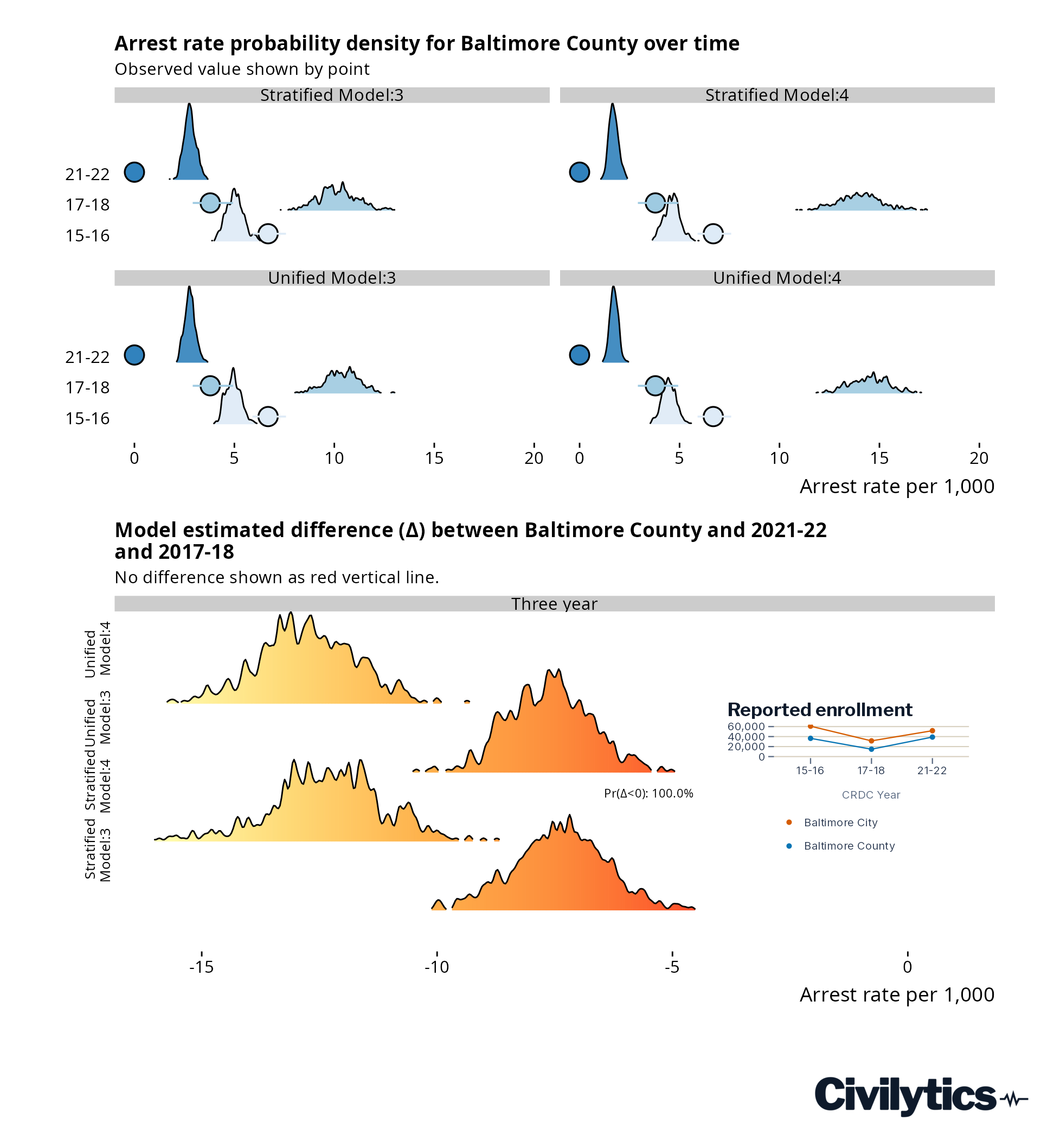
To better understand what is going on we can use our models to make temporal comparisons in Baltimore County - what does the trend look like.
We can
State-level overview
            used   (Mb) gc trigger   (Mb)  max used   (Mb)
Ncells   4793619  256.1   15070707  804.9  29434972 1572.0
Vcells 144981148 1106.2  425250724 3244.5 531563027 4055.6
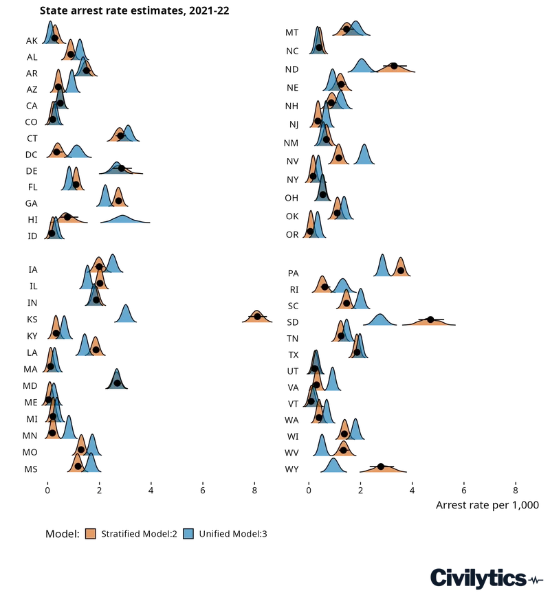
The recreation of the Table 1 state demographic-group differences is now part
of the white paper’s “Comparing state-level demographic group differences”
(wp_fig_state_differences); only the all-states overview above is kept here.