Abstract:
School-based punishment and discipline can be enormously consequential for students’ lives. Researchers have documented racial disparities in all outcomes along the school punishment continuum with Black students overrepresented among those experiencing every form of school punishment, including school-based arrests. To date, most public-facing analyses of school-based arrests focus on observed counts or rates with some exclusion restrictions based on sample size. These analyses quickly draw attention to outliers (some of which are data errors) and have limited use in making direct geographic, demographic, or temporal comparisons. Bayesian hierarchical models of rare events have been used to improve accuracy of rate estimates in a wide variety of fields. We show that by using this strategy we can greatly increase the ability to draw comparisons in arrest rates by increasing the rates’ precision. We evaluate the tradeoffs of several different model specifications of arrest rates in terms of precision and coverage and include applied examples of using model predictions to make informed comparisons.
Keywords: school-based arrests, racial disparities in school discipline, Civil Rights Data Collection, small-area estimation, Bayesian rare event models, measurement error, rare event rate analysis
This research was supported by a grant from the American Educational Research Association which receives funds for its "AERA Grants Program" from the National Science Foundation under NSF award NSF-DRL #1749275. Opinions reflect those of the author and do not necessarily reflect those AERA or NSF.
Intro
School-based punishment and discipline can be enormously consequential for students’ lives (Bacher-Hicks et al., 2019; Gottfredson & DiPietro, 2011; Skiba et al., 2014). Punishment and discipline exist along a continuum from in-class warnings to detentions to suspensions and expulsions, with the most serious discipline being referrals to law enforcement and arrests. There is a strong link between experiencing school discipline and a range of key outcomes for early adults, from pursuing higher education to being charged with or convicted of a crime, and the link between school discipline and many outcomes (particularly criminal justice contact) is strongest for Black students (Davison et al., 2022).
Over the past several decades, researchers have studied patterns in school discipline and both theorized about and empirically examined the consequences of the “school-to-prison pipeline” (for examples, see Bacher-Hicks et al., 2019; Homer & Fisher, 2020; Skiba et al., 2014; Welch et al., 2022). Researchers have documented racial disparities in every outcome along the school punishment continuum with Black students overrepresented among those experiencing every form of school punishment (Darling-Hammond & Ho, 2024; Ward et al., 2021). However, the magnitude of race-based disciplinary gaps varies substantially across districts (Gopalan & Nelson, 2019) and school characteristics, including student racial composition and the diversity of teachers and school leaders, are associated with differences in disciplinary outcomes for Black and Latinx students (Welsh et al., 2025).
The district level is often the appropriate site of authority for the policies and procedures leading to school arrests and is where individual and collective actors (parents, students, school staff, and elected officials) can have the most immediate, direct, and demonstrable effect. Unfortunately, high-quality systematic data at the local level is often not accessible or is limited by practical and methodological issues that provide fodder for critics to dismiss the data as one-year anomalies or potential data errors. Most, if not all, public-facing analyses of arrest rates (for examples, see National Equity Atlas, n.d.; Whitaker et al., 2019) focus on “raw” or observed counts or rates with some exclusion restrictions based on sample size. These analyses quickly draw attention to outliers (some of which are data errors), leading critics to question the validity of the data as whole. Despite the Office of Civil Rights taking steps before, during, and after data collection to ensure good data quality, with over 17,000 districts reporting hundreds of data elements, it is not feasible to identify and correct every possible data error. Additionally, while using rates rather than counts provides a sense of scale and standardization, rates’ sensitivity to slight differences in counts magnifies differences that may not be substantively meaningful (sometimes called the base rate fallacy). Taken together, these issues inhibit equity analyses and efforts to push for change.
The Civil Rights Data Collection (CRDC) is the only source for data on school-related arrests for all the nation’s public schools and districts. The most recent data are from the 2021-22 school year. The CRDC defines a “school-related arrest” as “arrest of a student for any activity conducted on school grounds, during on-campus school activities (in-person or virtual), while taking school transportation, or due to a referral by any school official.” Previous studies examining arrest rates using the CRDC have focused on larger districts with more arrests, where rates can be estimated most confidently (Losen & Martinez, 2020). But many communities may have high or disparate student arrest rates and go unexamined due to sample restrictions. This limitation is a fundamental one: arrests are relatively rare so measuring them with precision requires a large number of trials, or, in this case, a large student population. However, each school district’s overall and student group populations are fixed, making disparities in this rare but highly consequential school action invisible for many student groups and places.
Fortunately, improving estimation of events in fixed population units has a long statistical tradition, perhaps most notably through the U.S. Census Bureau’s Small Area Income and Poverty Estimates (SAIPE) program (Bell et al., 2016; Rao & Molina, 2016; U.S. Census Bureau, n.d.). In this tradition, public health scholars have used statistical models to measure variation in the prevalence of health outcomes like obesity and tobacco use across small geographic units (Li et al., 2009; Zhang et al., 2011). Likewise, Bayesian hierarchical models of rare events, a form of small area estimation, have been used to improve accuracy of rate estimates in such disparate applications as oil spill risks and accidental fishery bycatches (Martin et al., 2015; Yang et al., 2013). In education data, the U.S. Census has been working to expand the SAIPE program to school districts to measure proportions of school-age children in poverty.
We explore the use of similar strategies to better measure rare event arrest rates in the CRDC, showing that these strategies increase the utility of arrest rate estimates by increasing their precision. More precise arrest rates allow for more useful comparisons among districts, between student populations, and over time. Demonstrating the value of CRDC data and the findings it makes possible is particularly important at this time given concerns that the data collection may not continue under the Trump administration.1
Prior Research on School-Based Arrests
Some actions necessitate excluding students from the school environment at least temporarily, and perhaps even arresting them for the safety of other students and staff. However, relatively few school-based arrests are for these serious actions. Several studies have found that over three-quarters of school-based arrests are for fighting or disorderly conduct and that serious crimes, such as robbery with a weapon or sexual assault, are quite rare in schools (Na & Gottfredson, 2013; Whitaker et al., 2019; Wolf, 2013).
Research shows that school-related arrests and exclusionary discipline affect the academic achievement of not only students who are punished but also their peers, even after controlling for schools’ overall levels of violence and disorganization (Perry & Morris, 2014). For example, students assigned to middle schools with a one standard deviation higher suspension rate are 15% more likely to drop out of school, 11% less likely to attend a four-year college, and 17% more likely to be arrested between ages 16-21, controlling for a range of factors (Bacher-Hicks et al. 2024). Perry and Morris (2014) call these the “collateral consequences” of discipline and theorize they result from a heightened sense of anxiety among students, decreased trust between students and staff, and disruption of the school community.
Racial disparities in school-based arrest rates have been repeatedly demonstrated using prior waves of the CRDC, including the 2015-16, 2017-18, and 2020-21 data collections, and using state-specific data sources (Darling-Hammond and Ho 2024; Whitaker et al. 2019; Welsh et al. 2025; Wolf 2013). Examining both the 2017-18 and 2020-21 data collections and measuring Black overrepresentation across six types of punishment (in-school suspension, out-of-school suspension, expulsion, corporal punishment, referral to law enforcement, school-related arrest) and with multiple comparison groups, Darling-Hammond and Ho (2024) find that Black students are overrepresented among those disciplined in 99% of the estimates.
Of course, both arrest rates and disparities vary across place. Studies have examined how arrest rates vary by state, district, county-level racial bias, and whether schools have police (Riddle & Sinclair, 2019; Weisburst, 2019; Whitaker et al., 2019). Anticipating that the federal government will move backwards on issues of school discipline (Williams & Wiley, 2025), and recognizing that a narrative of a “youth crime wave” (outstripping actual available data on youth offenses) has taken hold (Knight et al., 2024; Stephens, 2024), it is potentially more important than ever to accurately identify patterns of school-based arrests and inequalities at the local and state level. Systematic data collection and academic research have much to contribute to limiting the number of arrests in schools and reducing racial disparities, but the impact of this work on local activism is impeded by uncertainty in how to use existing measures of school-based arrests comparatively to understand disparities, geographic patterns, and trends beyond the descriptive counts reported.
Data
The CRDC is generally a biennial data collection. The most recent available data, released in January 2025, are for the 2021-22 school year. To this, we add data from two prior collections: 2017-18 and 2015-16.2 The CRDC includes 17,704 school districts in 2021-22; 89% of these districts have three years of data available. In models that incorporate multiple waves of data, we include all available observations, which is three years for most districts but one or two years in some cases.3 The number of school-related arrests declined over these three waves from over 62,000 school-related arrests in 2015-16 to 52,300 in 2017-18 to 34,846 in 2021-22.
Student arrests are rare. In 2021-22, 34,846 students were arrested at school, including 11,259 White students; 11,666 Black students; 9,146 Hispanic students; and 529 American Indian/Alaskan Native students.4 More Black students were arrested than White students despite there being three times as many White students as Black students enrolled in U.S. public schools. 22,919 male students were arrested along with 11,927 female students.
In addition to being rare, student arrests are also sparse. In 2021-22, 2,060 districts reported an arrest. This is only 11.6% of the districts in the data, which means the most common value for arrests, by far, is 0. However, this small proportion of districts enrolled 45% of all students – meaning that nearly half of all students attended a school district where a school-based arrest occurred.
Because of this rarity and sparsity, we provide a detailed description of how we construct arrest rates from two sets of variables in the CRDC: arrest counts and numbers of students enrolled. For the denominator in our rate calculation, we use enrollment counts for each school by race and sex. When we encounter reserve codes indicating data suppression or an issue with the data collection itself, we treat these as missing values since the enrollment number cannot be recovered from the public use files. These records are discarded from the analysis, and we have a dataset with one row per year-school-race-sex with a non-missing enrollment count. 5
Arrest counts are reported for 28 student groups based on students’ race/ethnicity, sex, and disability status. We focus only on rates by race/ethnicity and sex, not by disability status, due to exceptionally sparse data created by the (relatively) small number of students with disabilities.6 However, arrest counts are not reported independent of disability status. To create arrest totals by race and sex, we exclude variables of counts of student categories that cannot be disaggregated by race and sex. Unfortunately, arrests and referrals of 504 students7 are only reported disaggregated by sex, not by race, which means there is no way to include this category of students in race and sex subtotals. These exclusions remove 1,785 arrests and 1,691,865 students from the analysis in 2021-22 (3.3% of the total). This is the only student group excluded from our analysis at this stage.8
For arrest records with a reserve code, we treat the value as 0 and retain them.9 Districts that reported enrollment data but did not report law enforcement data are thus preserved in our analysis. We hypothesize that, among districts with missing law enforcement data, many are likely to have had 0 arrests. By retaining them in the data we can analyze how the model treats these 0 values and better generalize to the population.
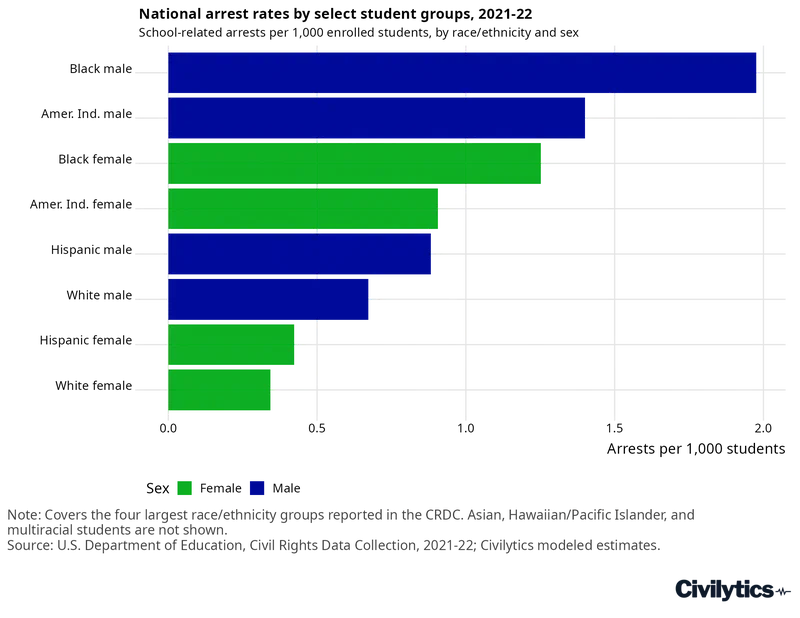
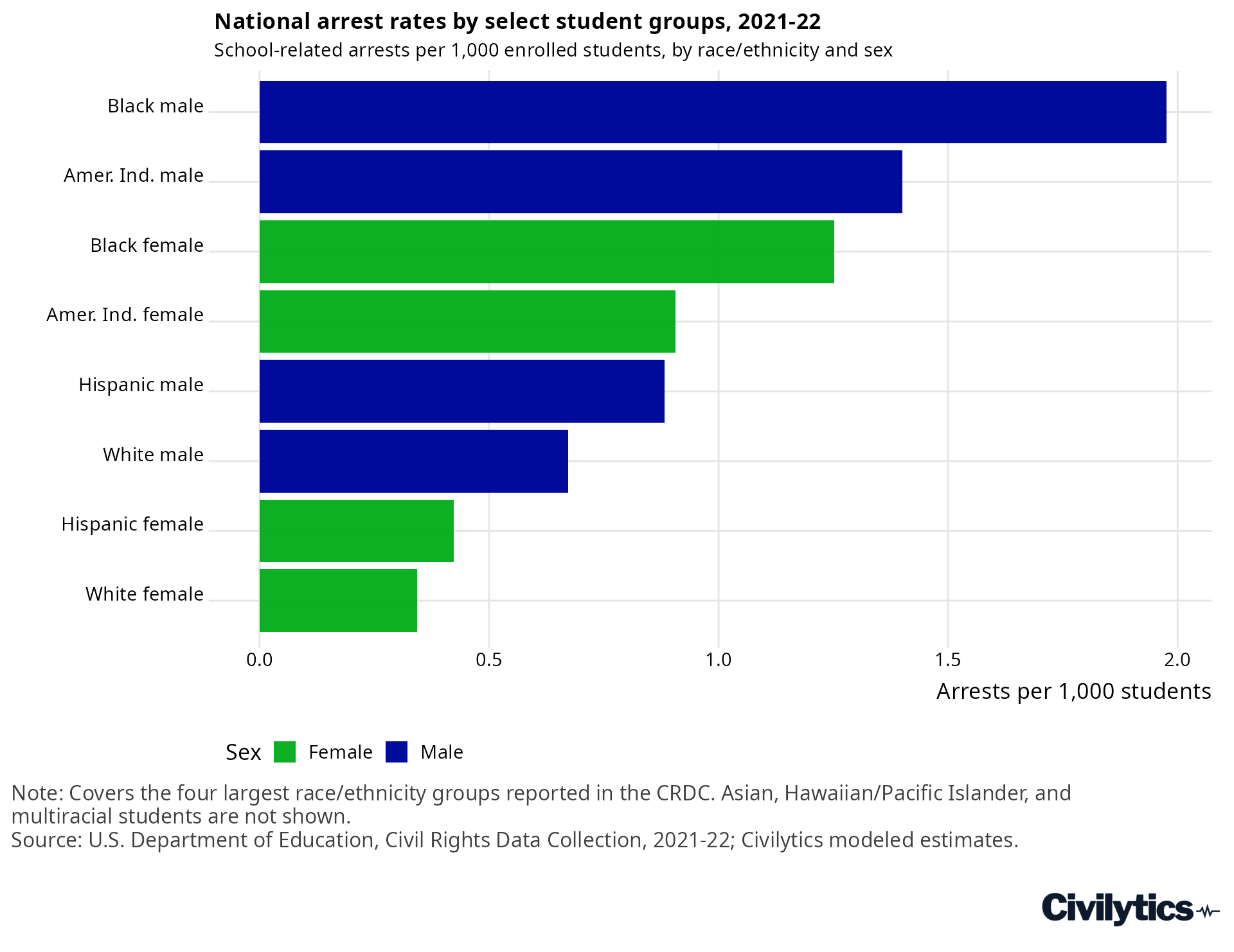
The result is a dataset with 48.6 million students enrolled in the schools included in the CRDC in 2021-22 and a national school-related arrest rate of 0.72 out of every 1,000 students. White students had 0.51 arrests per 1,000 students, Hispanic students 0.66, American Indian students 1.16, and Black students 1.62 arrests per 1,000 students. Male students had an arrest rate of 0.92 arrests per 1,000 while female students were at 0.50. The difference in the arrest rates of male and female students (0.42 difference) is smaller than the difference in arrests rates of White students and Black or American Indian students (differences of 1.11 and 0.65, respectively). Disaggregating by race and sex reveals even greater disparities: rates by student group vary from a high of 1.98 out of 1,000 Black male students to a low of 0.34 out of 1,000 White female students. These are shown in Figure 1 below.
We include “referrals to law enforcement” as a predictor. Referrals to law enforcement are defined as “an action by which a student is reported by a school official or that official’s designee to any law enforcement agency or official, such as a school police unit, for an incident that occurs on school grounds, during school-related events (in-person or remote), or while taking school transportation, regardless of whether official action is taken.” Data on referrals is reported at the same level (school) and in the same manner (by race/ethnicity, sex, and disability status) as arrest data and we treat reserve codes in these variables the same. Like arrests, the number of referrals also declined across the three waves of the CRDC we use, although much less dramatically.
We join the CRDC school counts to the Common Core of Data (CCD) school directory data for the same years to ascertain the grade levels served by each school. Schools in the CRDC but not in the CCD are excluded.10 Because younger (e.g., elementary age) students are rarely arrested, we exclude all schools that do not enroll students in grade 7 or above from our modeling analysis—we focus on modeling arrests for older students to avoid overly inflating the model toward schools with 0 arrests and to help speed up computation. The data thus includes junior high/middle schools, high schools, and K-8 or K-12 schools.11
Finally, since discipline and safety policies are usually set at the district level, we aggregate the data from schools up to districts. This increases our sample density (arrests and students per row) and reduces the number of rows in our dataset, making our arrest rate measurement more precise and our statistical models easier to fit. When fitting our models, we restrict the sample to districts that enroll at least 30 students total,12and we exclude any district student-group observation where the enrollment of that group is 0.
Motivation
There are two ways to interpret arrest rate data. The first is to take the data at face value—as a population. The CRDC is intended to be a population-level collection. In this interpretation, if we want to know the change in arrests from one year to the next, we simply subtract one year’s values from the next’s. The second approach is to treat the data as a measurement. A common use of arrest data may be to ask if a school district is likely to have a lot of arrests in the present, given the number of arrests they had in the past. In this interpretation, we need to understand the precision of the measurement so that we can determine if a change in arrests from one year to the next is greater than the difference we would expect due to random variance and/or measurement error. While the CRDC is intended to be a population-level collection, in fact, we know that nonresponse and reporting errors can lead to significant changes in the data independent of changes in those phenomena in schools, motivating a measurement approach.
Treating arrest rates as having measurement error has three distinct advantages, advantages that are increasingly important the smaller the population we measure (e.g., a school district). First, it allows us to quantify our uncertainty about the arrest rate to help us decide how confident we are in observed demographic, geographic, and temporal differences. Second, it reflects the data generating process of the CRDC, which, as we described above, is an impressive but imperfect effort to collect population-level statistics about all public schools. Third, it allows us to use statistical tools to improve our descriptive understanding of school-based arrests.
Unfortunately, the rarity and sparsity of arrests present us with two difficult challenges. First, estimating rare event rates in anything but very large populations leads to great uncertainty in the estimate. Since school districts are of a fixed population size and we are interested in annual data, we cannot increase the number of trials (students enrolled) to increase the precision. Second, arrest data are also sparse; because many district-student groups have far fewer than 1,000 students, we expect, and find, that 0 arrests is the most common observed value. However, those 0 values can have different meanings: that the school district never makes arrests, that there were insufficient students for the arrest rate to result in an arrest this year, or that there was an issue with the data reporting.
The classical approach to handling these challenges is to apply two statistical corrections: first, to construct an approximate binomial confidence interval for the rate, and second apply a correction to estimate the event rate in the case that the data are censored (no event is observed). To construct an appropriate binomial confidence interval around our arrest rates, we use the Agresti-Coull approximation, where the 95% interval is calculated by simply adding 2 trials and 2 failures to the observed data and computing the Wald interval (Agresti & Coull, 1998).13 In cases where 0 arrests are observed, we need a further correction to avoid a 95% interval of 0 – 0. In these cases, we apply the “Rule of Three,” which states that the 95% confidence interval for an event which has not occurred in the sample is defined as the range from 0 to where n is the number of trials observed (Hanley & Lippman-Hand, 1983). Essentially, we add 3 events to the data. This allows us to measure our uncertainty about the likelihood of the event probability given the truncated number of trials. It has been found to work well even with as few as 20 trials (Eypasch et al., 1995).
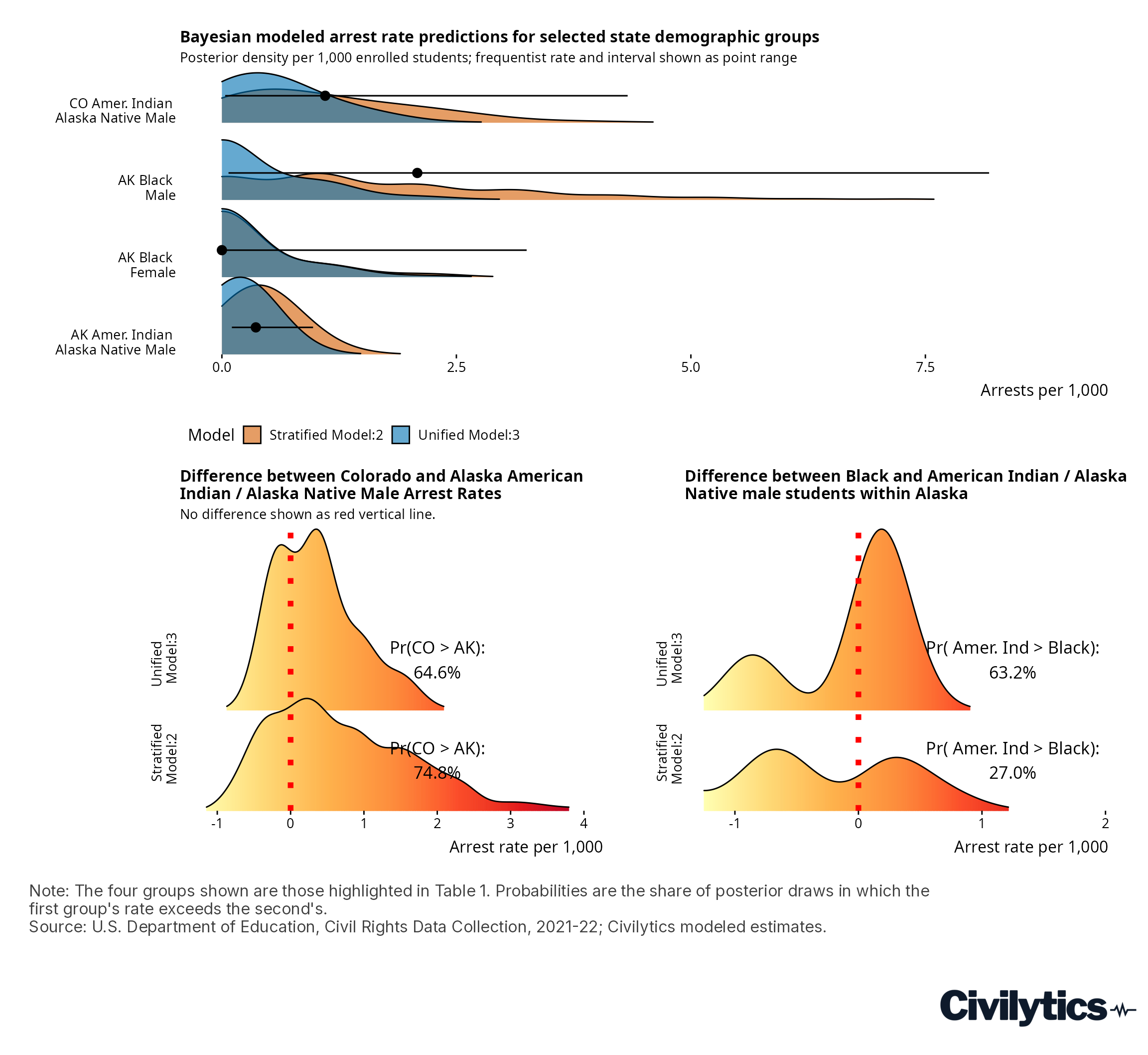
Unfortunately, this classical approach has limitations in cases of extremely rare events. To show this, let’s look at how this approach works in four cases of state student-group arrest rates from the 2021-22 CRDC. Table 1 shows the arrest rate and the Agresti-Coull approximate 95% confidence interval for the rate for four student groups. The rate and interval are adjusted to be per 1,000 students.
| Observation | Arrests | Enrollment | Rate per 1,000 | 95% interval (per 1,000) |
|---|---|---|---|---|
| AK Black Female | 0 | 922 | 0.00 | 0 – 3.25 |
| AK Amer. Indian Alaska Native Male | 4 | 11052 | 0.36 | 0.11 – 0.97 |
| CO Amer. Indian Alaska Native Male | 2 | 1816 | 1.10 | 0.04 – 4.33 |
| AK Black Male | 2 | 960 | 2.08 | 0.07 – 8.18 |
Table 1: Illustrating four sample state arrest rates
In comparing the first two rows of the table, we see that, after we apply the “Rule of Three” for the case with 0 arrests, the 95% interval for Black male students completely overlaps the interval for Black female students, despite the large difference in their observed arrest rates. Based on these confidence intervals, we cannot rule out that there is no difference between these student groups. Moving to rows 3 and 4, we compare across states and across two populations with very different enrollment sizes but with a difference of only two observed arrests. Colorado American Indian / Alaska Native male students have a much higher observed rate of arrest than their Alaskan counterparts. However, the Colorado arrest rate is based on a much smaller population and so has a much wider 95% interval, which completely encompasses the Alaskan student interval. In fact, while we may be tempted to interpret this table by saying that the Alaskan American Indian male students in row 3 are different because of their much narrower interval than all other student groups in the table, this would be incorrect. We cannot interpret “most likely values” within these intervals, so, although the Alaskan American Indian male interval only ranges from 0 to 0.79, we cannot determine the probability that this arrest rate truly differs from the other groups in a meaningful way since all the other intervals still encompass it.
This example table illustrates that—even at the level of state student group arrest totals—our assessment of rate differences is impaired. The problem becomes significantly worse when we look at individual school districts. If we are going to get meaningful information from arrest rates for the purpose of comparing across groups, geographies, or time we need to reduce our uncertainty in these measures beyond what is available to us in a classical approach. Thankfully, Dixon et al. (2005) identified several strategies that can meaningfully increase the precision of rare event rate estimates without the collection of additional data – with Bayesian statistical modeling showing promise. We follow the subsequent work of public health, environmental, and ecological scholars (Li et al., 2009; Martin et al., 2015; Yang et al., 2013; Zhang et al., 2011) and turn to Bayesian hierarchical models of rare events, a form of small area estimation.
Bayesian multilevel modeling is appealing because it not only can help us construct prediction intervals for the arrest rates but can also regularize our rate estimates using information about the whole dataset, taking advantage of the hierarchical structure of student groups within districts within states. This has the potential benefit of reducing the impact of reporting errors and outliers. Additionally, we can use posterior draws from the Bayesian model to construct uncertainty intervals around any quantity of interest – such as differences in arrest rates between student groups. Of course, to achieve this, these statistical models bring in assumptions about how observations in the data are related and how predictors are related to our outcome of interest. Next, we describe the specific model specifications we will explore, the assumptions they encode, and how we expect them to impact our estimation of arrest rates.
Methods
We divide our investigation into two parts: 1) fitting unified models to the entire dataset, and 2) fitting stratified models for each demographic group independently. In both cases, we fit five model specifications with increasing complexity. In the unified models, due to computational constraints, we allow district arrest rates to vary but assume that demographic group disparities within districts are constant nationwide. In stratified models we allow district-student group rates to vary, but the models treat every district-student group independently and do not use information about other student groups within the same district. The five specifications we compare are shown in Table 2.
| Specification | State and district random effects | Level 1 covariate | Level 2 covariate | Prior years of data |
|---|---|---|---|---|
| 1 | X | |||
| 2 | X | X | ||
| 3 | X | X | ||
| 4 | X | X | X | |
| 5 | X | X | X | X |
Table 2: Model specification summary
For all models, we use a repeated measures structure where each combination of race and sex constitutes a row in the dataset and the number of students arrested and students enrolled in that group represent our binomial outcome. We then model the arrest outcome as where is the observed number of arrests in the student group within the school district, is the number of students in that student group, and is the estimated arrest rate.14
Model 1: A Bayesian multilevel model
For our baseline unified model, we model the 2021-22 district level arrest rates with random intercepts for state and district. The arrest rate, , is modeled using as a linear multilevel model. The rate for each district-student group is modeled as a combination of a state-specific random intercept, , a district-specific random intercept, , district-student group specific predictors , and a district-student group error, .
In the case of the stratified model, Model 1a below, instead of , we fit the model to each subset of the data, allowing the state and district random intercepts to be estimated independently for each group. For all remaining specifications, the stratified model can be represented similarly to Model 1a with the addition of the same non-demographic covariates as are added in each unified model. In both the unified and stratified versions, the model shrinks arrest rates toward the district, state, and grand mean when is low – but in the unified model that grand mean is pooled across all student groups, while, in the stratified model, it is student group-specific.
Model 1a: Stratification by student group
We start with Model 1, and not a simpler model without state-level effects or demographic group fixed effects because, while an even simpler model would be easier to fit, it would not address student group-specific differences that motivate our interest in recovering arrest rates in cases of rare events. This model also serves as a useful benchmark to evaluate the tradeoff of additional modeling complexity in terms of additional assumptions, complexity to fit, and data requirements.
Our first addition is a level 1 district-student group covariate for the referral rate to law enforcement for each student group. This model estimates arrests conditional on the rates that students are referred to law enforcement from each student group. In selecting this predictor, we theorized that school disciplinary actions are a continuum of increasing punitiveness and that events closer on the continuum are more strongly correlated. Since including multiple predictors incurs penalties in interpretability and data availability, we selected the measure most closely related to arrest rates (referrals to law enforcement) rather than one “earlier” on the continuum (e.g., suspensions) which may have resulted in additional data loss from missing records.
Model 2: Bayesian multilevel regression model with covariates
Models 1 and 2 evaluate the effectiveness of modeling on a single wave of CRDC data alone. For models 3 through 5 we explore the impact of adding additional years of data. Our first multiyear model, Model 3, is identical to Model 1 except it is fit to CRDC data from 2015-16, 2017-18 and 2021-22, and includes a fixed effect for each year, to account for national annual differences in the arrest rate. The result is that for most districts and student groups, we have three observations of arrest and enrollment counts from which to estimate the arrest rate.
Model 3: A Bayesian multilevel model with multiple years of observations
Like Model 3, Model 4 includes three years of CRDC data; it also incorporates the district-student group covariate for the rate of referrals to law enforcement that was used in Model 2.
Model 4: A Bayesian multilevel model with multiple years of observations and covariates
Finally Model 5 adds a district-level (level 2) covariate, , for the total number of referrals to law enforcement in that district each year. This allows us to estimate the district-level arrest rate intercept conditional on the total referrals, estimated as a fixed effect . We can only include level 2 covariates in the case of multiple years of data since, in a single year, any district-level covariates would be perfectly collinear with the district random intercept, We use this model to explore how much of the variance in district-level arrest rates can be explained by district-level law enforcement referral rates and if this improves model performance.
Model 5: A Bayesian multilevel model with multiple years of observations and covariates
In all models, we log-transform our level 1 and level 2 covariates to align the scale with our outcome variable and improve the speed of the MCMC sampling algorithm. We use weakly informative, or regularizing, priors which constrain the parameters to the plausible range given the scale of our measurements (Chung et al., 2015; McElreath, 2020).15
Without computational limits, we would ideally fit a sixth model that adds district-level random slopes for race and sex to model 5 to allow us to model the within-district variation in student group arrest rates directly.
Hypothetical Model 6: Full Bayesian multilevel regression model with district effects
By allowing the effect of race and sex on arrest rates to vary by district, this model would align with our understanding of the data and prior research on arrest rate disparities but is computationally unfeasible. It would require estimating 136,000 additional parameters, each with at most three rows of data support—the vast majority without any observed outcome (arrest). This combination of size and sparsity makes such a model impossible to reliably compute presently.
As a compromise, we fit stratified versions of models 1 through 5. Our descriptive analysis of the arrest data shows that Dixon et al.’s criteria for stratification to improve rare event precision are easily met, namely: strata (race and sex) are defined exogenous to the response variable, event probabilities vary markedly between strata, and the size of each stratum is known (2005). For the stratified models, we fit each of the specifications 1-5 eight times, once each for these student groups: Black male, White male, Black female, White female, Hispanic/Latino male, Hispanic/Latino female, American Indian male, and American Indian female. This results in a total of 40 models, which is why we focus on only eight specific student groups instead of all 14 possible combinations in the data (i.e., we do not fit models for Asian students, Hawaiian/Pacific Islanders, or multiracial students). We then present the combined results from all of the data subsets for each specification in the tables of results below.
While the specifications are similar for the unified and stratified models, we expect the results to be very different. The unified models assume that districts as a whole vary in their overall arrest rates, but that variation among student groups within the district is constant across the country—that is, the effect is fixed. This is a useful assumption that both allows us to fit models and allows us to compare observed values to a counterfactual that student group disparities within districts do not vary greatly. The stratified models allow us to test that assumption by fitting separate district intercepts for each student group, allowing student group variation to vary by district. The drawback is that working with eight models jointly instead of a single unified model is more complex, and the number of observations for each district-student group intercept is greatly reduced, which should result in less precise estimation. We explore the implications of these differences below.
Model Comparison
Following Rohrer & Arel-Bundock we are evaluating our models as “prediction machines”—that is, we are focused on how well these models generate predicted values that assist us in understanding differences in rare event rates (2025). These are not causal models. Therefore, we want to assess how well models allow us to draw policy-relevant conclusions. To do this, we assess models on two criteria: coverage of the reported arrest rates and precision of the arrest rate estimate interval.
We compare each of our Bayesian models to the approximate binomial proportion confidence interval measured by the Agresti-Coull approximation and use of the Rule of Three described above, which we refer to as the frequentist interval. For Bayesian prediction intervals for each model, for each district-student group arrest rate, we calculate the median fitted value and the lower and upper bounds of the 95% highest-posterior density (HPD) interval from 500 draws from the posterior. To calculate precision, we take the standard deviation of these 500 draws.16 We then present comparisons for four specific metrics:
Coverage: in what % of observations does the 95% prediction interval overlap the observed value in the data
Median precision: the median of for all values; the higher this value, the more precise our arrest rate estimate and the narrower our prediction interval. We prefer the median to the mean because of the skewness of the distribution that results from the large number of cases with 0 arrests.
Narrowed intervals: in what % of observations is the modeled 95% interval equal to or narrower than the frequentist interval
Median % narrowed: what is the median percentage change between the modeled interval and the frequentist interval
Because we are interested in the practical applications of applying models to rare events to better facilitate demographic, geographic, and temporal comparisons, we present results for four relevant subsets of the 2021-22 CRDC data. We hypothesize that models may have different patterns of coverage and precision depending on the size of the student group and the magnitude of the observed arrest rate—these data subsets allow us to examine to what extent that is true. The different subsets are:
The full sample
Districts with an observed arrest
The 100 districts with the most total arrests
The 100 largest districts with 0 total arrests
Results from the full sample evaluate models across the range of arrest rates (from 0 up) and how each model is impacted by the relative sparsity of arrests across observations. The second sample illustrates how models perform in cases where the rule of 3 is not applied and we are only comparing our Bayesian models to the Agresti-Coull approximation. The third illustrates how the models compare when arrests are very frequent, sometimes suspiciously so. The fourth looks at the opposite issue where the district is large enough that we expect to observe an arrest and do not. We report all results on the most recent year of data (2021-22).
Our expectation is that the unified models will have worse coverage but greater precision than their stratified counterparts. We also hypothesize that models 1 and 2 fit to one year of data will have higher coverage, but wider intervals than model 3 through 5 fit to multiple years of data. We expect our limited covariates (Models 2, 4, and 5) to provide some improvement in terms of more precise intervals, but to not be as significant as additional years of data (Models 3 through 5).
In addition to our expectation that the Bayesian intervals will have good coverage and improved precision, they have two other distinct advantages. First, the Bayesian approach has a more satisfying interpretation: the Bayesian prediction intervals we construct represent the intuitive interpretation of prediction intervals—that there is a 95% probability that the true arrest rate lies between the boundaries of the interval. The confidence interval does not have this straightforward interpretation, though it is often treated as such (Gelman & Hill, 2006). Second, by using models, we can construct prediction intervals for any comparisons we wish to make, such as comparing arrest rates between student groups in a district, across districts, or within a district over time. We can use the draws of the posterior distribution to instantly calculate the average difference, its most likely interval, and visualize the results. We close the paper with some applied examples illustrating how these properties of model prediction intervals aid our interpretation of arrest rates for specific districts.
Results
The results show that fitting Bayesian hierarchical models to arrest rates can increase the precision of rate estimates while maintaining high coverage of the observed rate. This has practical applications, allowing rare event information to be useful in decision making, even in the case where the population is small relative to the frequency of the event.
Full sample results
Our first set of results are for the 2021-22 analytic sample for all districts and student groups. For these results, it is important to remember that the vast majority of observations (>95%) have an observed arrest rate of 0 – which makes distinguishing among models challenging.17 Still, differences emerge. Model coverage of the observed results is 100% in the one-year stratified models (stratified models 1 and 2). This is as expected, as the stratified models have only one row of data per observation and can only adjust the observed values by estimated state averages and the number of referrals. The unified one-year models (unified models 1 and 2) come close to this coverage, but, for a small number of observations, their expected arrest rate does not include the observed value. In these cases, for these models, the district-average of all student groups has pulled one or more student group estimates away from the reported rate – we can say the prediction is attenuated by other arrest rates within the district. In all cases, models with three years of data (models 3 through 5) have slightly lower coverage because the same process of attenuation can occur by arrest rates from prior years of data for all observations. We will return to this phenomenon in other sets of results; if we believe there are mismeasurements of arrests in the 2021-22 data and that arrest rates are autocorrelated over time within districts, then this reduction in coverage may be a strength.
Using the second metric we compare the precision of arrest rate estimates and see greater differentiation across models – but we must be careful to interpret it. In this sample, the frequentist median observed precision is 0.384, which is for a district with 0 arrests. In this case, we see that all the models substantially improve precision in cases where no arrests are reported, as the median modeled arrest rate precision ranges from 2.44 to 8.32. However, the pattern within the unified models shows that adding predictors (going from model 1 to 2 and model 3 to models 4 and 5) decreases precision, while for stratified models adding predictors increases precision. We will explore this pattern across the various subsets to better understand differentiation among the models.
Our third metric is intended as a more practical take on the median precision. We tally observations that have a modeled interval equal to (i.e., no larger than) or better (i.e., narrower than) the frequentist interval. All models fit to one year of data had a slightly higher percentage of “equal or better intervals” compared to three-year models. In both the unified and stratified models with three years of data adding a level 1 covariate (moving from model 3 to 4) improved the percentage of “equal or better” intervals by about 1 percentage point, but the addition of a level 2 covariate did not provide further improvements.
Our fourth metric should illustrate the differences between the models in more detail by measuring the median shrinkage of the 95% interval around the rate expressed as a percentage of the frequentist interval width. However, in the case of the full sample, the median value of arrests is 0, so the frequentist interval is defined by the rule of three and is quite large. In most of these cases, the Bayesian models are constructing a 95% prediction interval composed entirely of 0 arrests because that is consistent with what we would expect for small samples (that is, we would estimate with 95% probability or higher that there were 0 arrests). The large proportion of these cases leaves little room for the models to differentiate from one another on this metric.
Overall, looking at the full sample, we can conclude that the modeling “worked” to improve precision without sacrificing coverage of the true value: nearly all prediction intervals are narrower than their frequentist counterparts. However, simply looking at the averages masks some important differences in how each of the models addresses patterns in the data, so we now turn our attention to comparing these metrics for specific subsamples of interest.
| Models | Coverage | Arrest rate precision (median) | % equal or better intervals | Median % narrowed |
|---|---|---|---|---|
| Unified 1 | 99.7% | 8.56 | 98.8% | 100.0% |
| Unified 2 | 99.9% | 6.70 | 99.0% | 100.0% |
| Unified 3 | 98.3% | 5.97 | 97.8% | 100.0% |
| Unified 4 | 99.2% | 5.14 | 98.5% | 100.0% |
| Unified 5 | 99.2% | 5.17 | 98.5% | 100.0% |
| Stratified 1 | 100.0% | 2.47 | 98.7% | 100.0% |
| Stratified 2 | 100.0% | 4.45 | 98.4% | 100.0% |
| Stratified 3 | 98.8% | 2.43 | 97.6% | 100.0% |
| Stratified 4 | 99.4% | 4.05 | 98.3% | 100.0% |
| Stratified 5 | 99.4% | 4.26 | 98.3% | 100.0% |
Table 3: Model results for full sample
Number of rows of data = 106,703. Observed precision = 0.384 calculated from the Agresti-Coull approximate interval with the rule of three applied.
District-student groups with an observed arrest
Because the prevalence of 0s makes it difficult to evaluate models, it is important to ask how our models compare to each other and the frequentist interval when an arrest is reported. The first big difference is that coverage has declined with only one model achieving 100% coverage (stratified model 1) and the unified multiyear model (unified 3) having only 72% coverage of observed arrest rates. The drop in coverage is attenuated by the addition of covariates, with improved coverage occurring between models 1 and 2 (except in the stratified case where model 1 already achieves 100% coverage) and among model 3 and models 4 and 5. Our chosen covariates, law enforcement referrals, are moderating the prediction intervals back toward the fitted values in these cases – increasing coverage.
The two most important distinctions in these results in Table 4 are that moving from one-year to multiyear models greatly decreases coverage, and moving from no covariate to a covariate improves coverage but reduces the median amount of shrinkage of the intervals. With the exception of stratified models 1 and 2, which appear to be too similar to distinguish, we see that adding years of data in models 3 through 5 reduces coverage, but shrinks our interval estimates on average by significantly more – giving us more precise intervals that in a higher number of cases disagree with the observed data. These results align with our expectations that more years of data can help shrink intervals but may miss the current year of data’s observed value in the case of high within-district student group variance in arrests across years. However, the addition of covariates can greatly reduce this effect, increasing coverage by almost 10 percentage points in the stratified models and over 13 percentage points in the unified models.
In other words, in this sample, we can trade some coverage for much greater precision in the intervals of our arrest rates by choosing a multiyear model. Depending on the use case, this tradeoff may be desirable. Adding covariates to the multiyear models can strike a middle ground, returning some of the coverage lost by adding multiple years, but also providing narrower intervals than one-year models.
| Models | Coverage | Arrest rate precision (median) | % equal or better intervals | Median % narrowed |
|---|---|---|---|---|
| Unified 1 | 94.3% | 4.30 | 82.2% | 37.3% |
| Unified 2 | 97.8% | 3.92 | 82.9% | 36.1% |
| Unified 3 | 72.3% | 4.43 | 89.3% | 54.2% |
| Unified 4 | 85.4% | 4.66 | 89.5% | 48.7% |
| Unified 5 | 85.5% | 4.55 | 89.5% | 48.7% |
| Stratified 1 | 100.0% | 2.23 | 70.4% | 23.4% |
| Stratified 2 | 99.5% | 2.36 | 69.5% | 23.2% |
| Stratified 3 | 80.4% | 3.71 | 87.8% | 52.9% |
| Stratified 4 | 89.0% | 4.81 | 84.9% | 42.9% |
| Stratified 5 | 89.2% | 4.65 | 84.6% | 42.7% |
Table 4: Model results for sample of district-student groups with an observed arrest
Number of rows of data = 4,729. Observed precision = 1.89 calculated from the Agresti-Coull approximate interval.
100 districts with most total arrests in 2021-22
Now we look at the results for all student groups for the 100 districts with the most total arrests. Here, we expect modeling to have the least utility because the rare event is much less rare. In this subset, the median precision of 2.74 is more than 7x greater than in the full sample alone, which means the frequentist intervals will be narrower and better performing.
Again, some interesting patterns emerge. First, our stratified one-year models continue to be the best at coverage, with perfect scores. Our unified one-year models have lower coverage than the stratified models, though the inclusion of a covariate in the second model improves coverage by nearly 10 percentage points and approaches the stratified models with 95.7% coverage. Among the one-year models, looking at precision, the stratified models improve on or equal the frequentist interval in fewer than half of all observations and on average they inflate the interval of the rate estimate by 14.8% to 16%. The unified models fare better, having other rows of the same district to attenuate their estimates by, but they equal or beat the frequentist interval in fewer than 2/3 of observations and the median improvement in interval width is less than 10 percentage points.
Among the multiyear models 3-5, the pattern of coverage is similar with adding a covariate providing a substantial increase in coverage from 59.2% to 75.3% in the unified models and 62.8% to 82.1% in the stratified models. This suggests that the data on law enforcement referrals strongly reinforces the data on arrests and pushes estimates closer to the reported data. However, in multiyear models the addition of this covariate – as we saw in the previous section – inflates intervals making the improvements in precision more modest for models 4 and 5 compared to model 3.
| Models | Coverage | Arrest rate precision (median) | % equal or better intervals | Median % narrowed |
|---|---|---|---|---|
| Unified 1 | 86.5% | 1.69 | 60.3% | 7.5% |
| Unified 2 | 95.4% | 1.98 | 63.9% | 10.3% |
| Unified 3 | 58.5% | 2.71 | 87.2% | 38.5% |
| Unified 4 | 75.4% | 2.30 | 83.7% | 27.2% |
| Unified 5 | 76.3% | 2.37 | 83.7% | 27.0% |
| Stratified 1 | 100.0% | 2.23 | 42.5% | -15.3% |
| Stratified 2 | 100.0% | 2.40 | 41.7% | -14.1% |
| Stratified 3 | 62.5% | 3.20 | 85.5% | 36.1% |
| Stratified 4 | 82.3% | 3.23 | 73.9% | 21.8% |
| Stratified 5 | 81.8% | 2.68 | 72.7% | 21.7% |
Table 5: Model results for 100 districts with most total arrests
Number of rows of data = 784. Observed precision = 2.74 calculated from the Agresti-Coull approximate interval with the rule of three applied.
100 districts with largest student enrollments but no arrests
On the other extreme of the data, we have very large districts with 0 reported arrests, which we call “suspicious 0s.” We selected the 100 largest districts with 0 total arrests. For these districts we calculate a “naïve” expected number of arrests based on the arrest rate per 1,000 students of the 100 districts with the largest student enrollments. The arrest rate for these districts is 1.15 per 1,000.18 Using this rate, and the assumption that all of the 0s are misreported, we would “naïvely” expect 2,645 arrests. We know it is unlikely that the true number of arrests in these districts was 0, and it is also unlikely that all of the districts simultaneously failed to report their arrests.
We evaluate how each of our model specifications approach this problem. In the table we compare the total arrests predicted for the districts by each model (total arrests predicted are the median, across posterior draws, of the predicted arrests summed over all district-student groups for each model), along with the 95% expected range of that summed total across draws.
| Models | Modeled arrests | 95% expected range |
|---|---|---|
| Unified 1 | 27 | 16 – 38 |
| Unified 2 | 41 | 29 – 58 |
| Unified 3 | 1,704 | 1,625 – 1,787 |
| Unified 4 | 810 | 753 – 870 |
| Unified 5 | 821 | 763 – 878 |
| Stratified 1 | 109 | 84 – 138 |
| Stratified 2 | 139 | 112 – 171 |
| Stratified 3 | 1,686 | 1,596 – 1,772 |
| Stratified 4 | 828 | 766 – 898 |
| Stratified 5 | 830 | 770 – 894 |
Table 6: Model results for 100 districts with largest student enrollments but no arrests
Number of districts = 100 (797 district-student groups).
These results align with our expectations: none of the models goes as far as the naïve approach and ignores the current data in favor of an alternative rate from similar districts. Just as importantly, none of the models estimates that there were 0 arrests. We also see familiar patterns emerge: multiyear models have higher expected arrests due to drawing on prior data. Adding covariates decreases (significantly) the number of missing arrests modeled. We also see there is not much difference between the models with a level 1 covariate and model with both a level 1 and level 2 covariate – continuing a theme that the level 2 covariate does not have a substantial impact on results. One surprise is that the stratified one-year models predict many more missing arrests than the unified models. This could be because of the wider intervals we saw in Table 5 leading to increased variability in the median arrest.
What is clear is that across all of the models the likelihood of 0 arrests for these 100 districts is less than 2.5% – that is, it is outside the 95% prediction interval. And, if we account for prior years of data, then as many as 1,794 and at least 751 arrests are missing from the 2021-22 CRDC in just these 100 districts.
Initial conclusions
Taken together, the results suggest we have options in how to use modeling to approach measuring arrest rates. If we are suspicious of outliers and errors in a specific year of reporting, we can choose a multiyear model knowing that some of our predicted values will differ from the reported values (reduced coverage). In doing so, we can include a covariate to more heavily weight the information in the current year (models 4 and 5) and increase our coverage but worsen our precision. Or we can use a model without covariates (model 3) and increase our precision but, by weighing prior years of data more heavily, suffer decreases in coverage.
For districts with higher average arrest rates, we should avoid using one-year stratified models because, in these cases, stratification does nothing to improve upon the frequentist intervals. However, the one-year unified models can provide high coverage and marginal improvement over frequentist intervals. How we choose among these options depends on the question we are asking, the districts we are investigating, and our prior beliefs about rates of error in the data collection and autocorrelation in arrest rates.
Applied Examples
Our purpose in understanding how model prediction intervals behave descriptively is to learn how we may use models to better understand rare event rates for subnational populations of interest. To demonstrate what we have learned we provide a few applied examples in which we compare model predictions to the frequentist interval calculated from the data.
A case study of zero reported arrests
The first example examines how Bayesian prediction models differ from frequentist intervals in a case of no observed arrests. The Paterson New Jersey school district has 18,310 students enrolled, so having 0 arrests is suspicious.
In the case of no arrests, the observed interval is constant – from 0 to 3 – and shown in gray alongside the Bayesian prediction interval in blue for each of our 10 models. The models are sorted into one-year specifications on the left and three-year specifications on the right. We see that the one-year models, except for stratified model 1, have much narrower intervals than the frequentist interval, confirming the advantage of the modeling methodology for increasing precision in cases without an arrest.
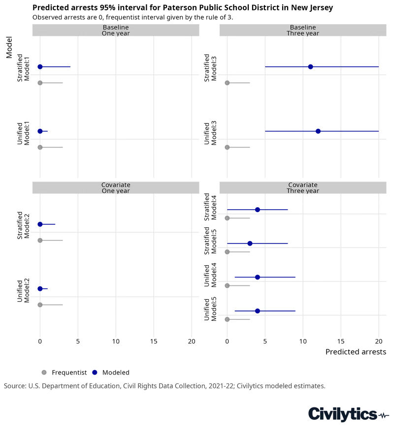
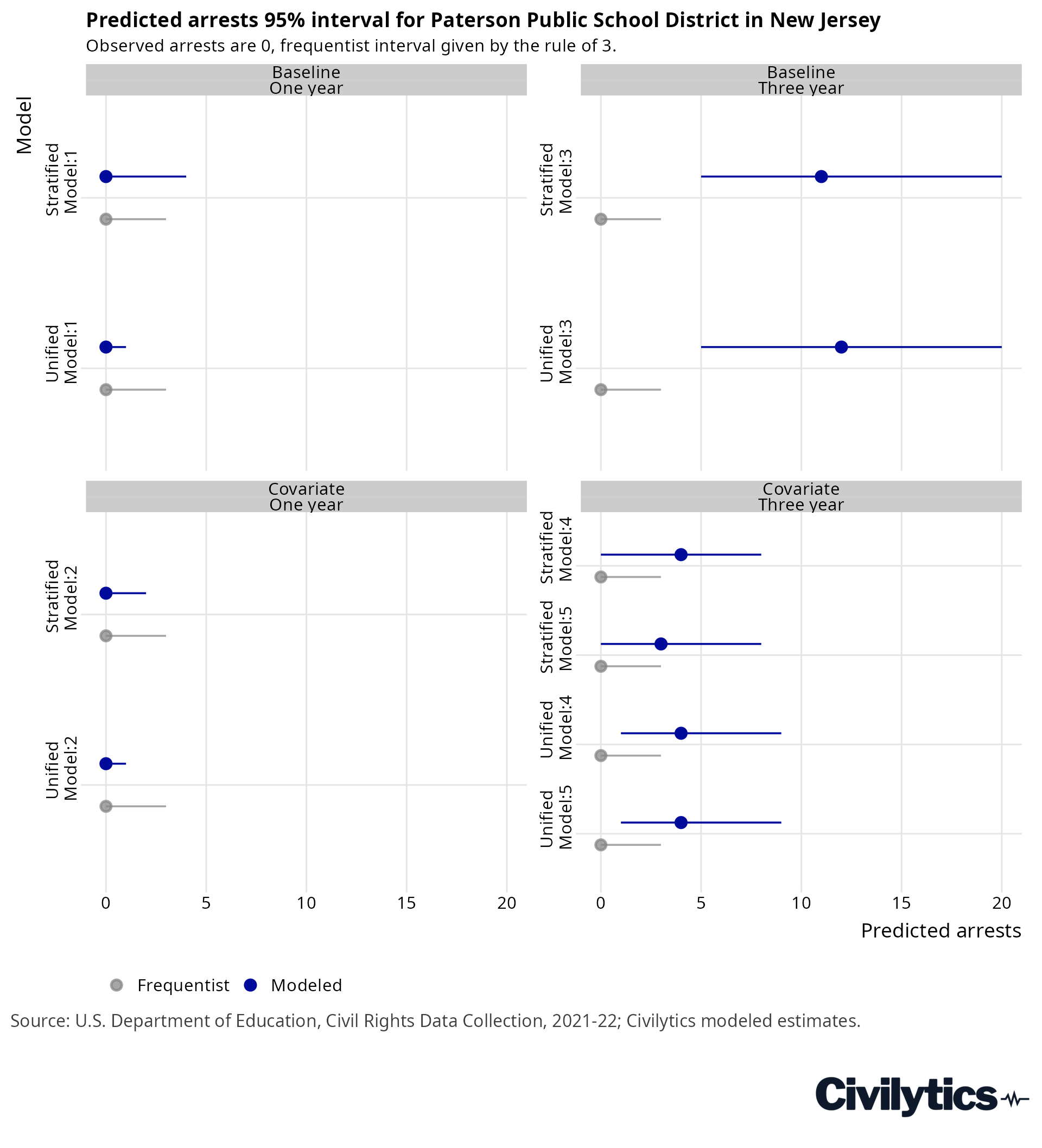
However, these models still suggest that 0 arrests is the median estimate (the point). Here the three-year models disagree. Intervals for the three-year models are all wider than the frequentist interval and the median estimated arrests is greater than 0. Models without covariates (model 3) suggest that more than 10 arrests are most likely. The reason becomes clear when we look at the underlying data and see Paterson reported 47 arrests in 2015-16 and 11 arrests in 2017-18. The three-year models are incorporating this information, which expands their intervals. But, with Bayesian models, we can go beyond simple point intervals, as we show in the next figure.
Here, every draw of the model is plotted as a histogram. For clarity, we show only the covariate specification with a level 1 covariate because there are almost no meaningful differences from the version with level 1 and 2 covariates.
The one-year models agree that 0 is the most likely arrest number for Paterson, but now we can quantify it differently. For example, the stratified model (top left) is less confident in 0 than the unified model, giving a near equal chance (47.2%) of greater than 0 arrests as 0 arrests. Adding a covariate brings the stratified model closer to the unified model, increasing the chance of 0 arrests to 76.4%. Interestingly, the covariate has much less effect on the unified model, only increasing the chance of 0 arrests from 82.2% to 84%. Even though these models are fairly confident that there are 0 arrests, they cannot rule out 1 arrest with 95% confidence (as we also saw in the point intervals in the previous figure).
Things are more interesting with the three-year models. Without covariates, these models are very confident that there are more than 0 arrests in Paterson, but uncertain about exactly how many, with a relatively flat distribution of likely arrest counts ranging from 8 to 15, and a substantial tail at 16 or more arrests (top right panel; note change in x-axis – arrest counts are truncated at 16 for visual clarity). These models confidently rule out 0 arrests and cannot confidently rule out as many as 16 missing arrests.
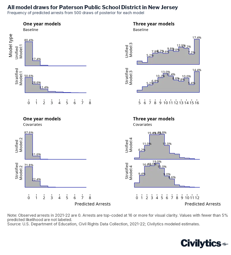
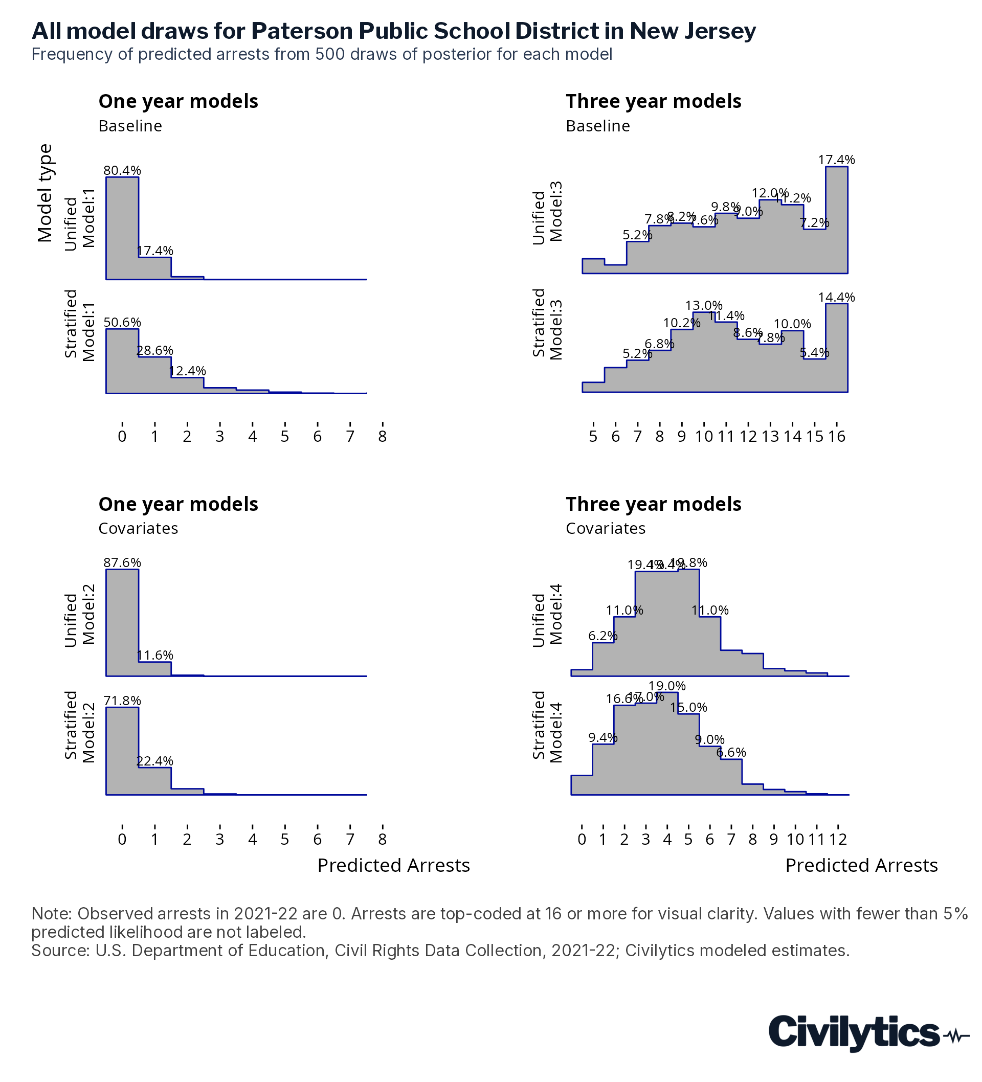
Adding covariates greatly changes the picture, shifting the distribution of expected arrests downward, with 3 to 4 arrests now being the most likely. These models still rule out 0 arrests with 95% probability but cannot rule out only 1 arrest. The three-year models all differ greatly from the one-year models, which we expect when incorporating the prior information about Paterson into the model. However, we also see that the impact of the covariates is substantial because in 2021-22 Paterson reported 0 referrals to law enforcement; this absence of referrals provides additional information to the model that the prediction should be pushed toward 0.
Taken together, these models give us three ways to think about the likelihood of 0 arrests in Paterson, New Jersey: strongly align with the reported data and improve precision over the frequentist interval (one-year models 1 and 2); strongly weigh the historic pattern of arrests in Paterson and expect 10 or more arrests (model 3); or find a middle ground between these two by taking into account the additional information we have from reported referrals (models 4 and 5). With Bayesian intervals we can choose the method that is most appropriate to our application.
A case study of many arrests
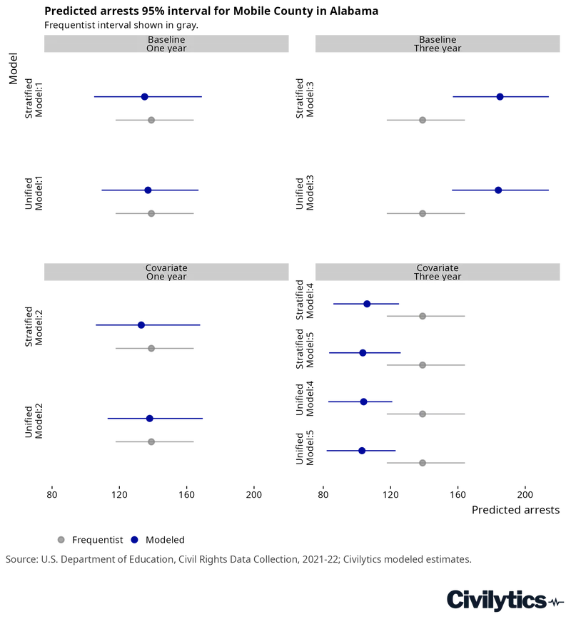
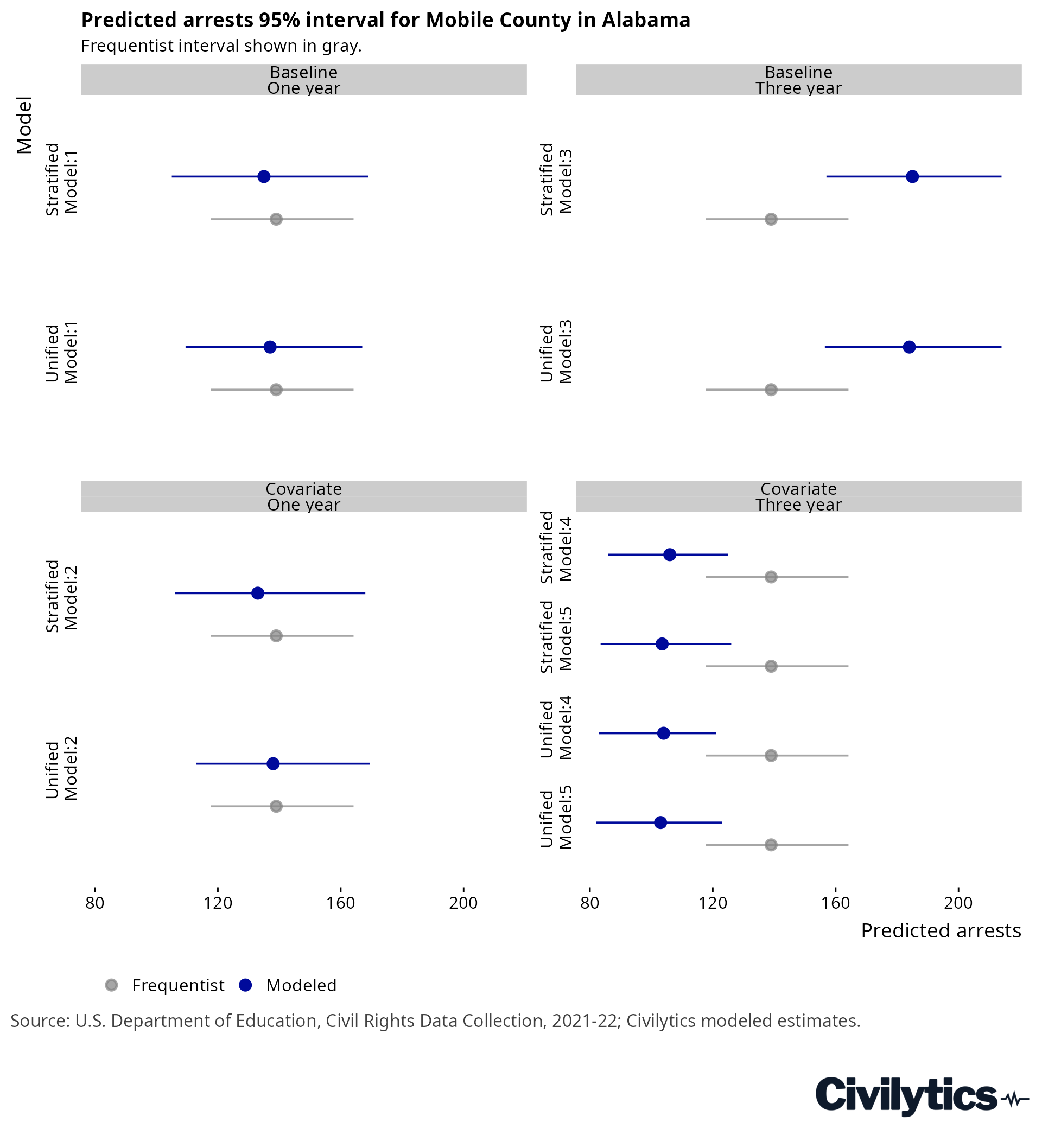
Now we turn our attention to the other end of the scale: how the models perform when there are many observed arrests. Consider the case of Mobile County, Alabama, a district with 25,745 students which reported 139 arrests (5.4 arrests per 1,000 students). In the figure below, in all models except unified models 4 and 5, the observed interval in gray is narrower than the modeled intervals in blue. Again, the biggest distinctions among models are between one-year models (left side), which closely track the frequentist interval but are wider; the three-year models without covariates (top right), which tend toward more arrests than the frequentist interval; and the three-year models with covariates (bottom right), which tend toward fewer arrests than the frequentist interval.
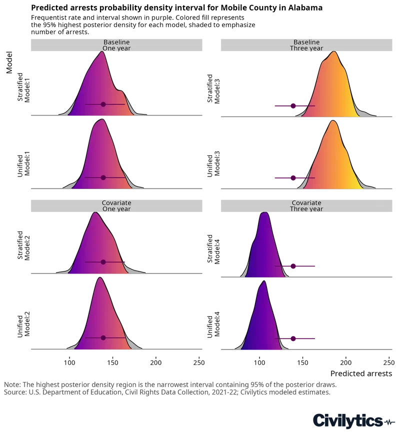
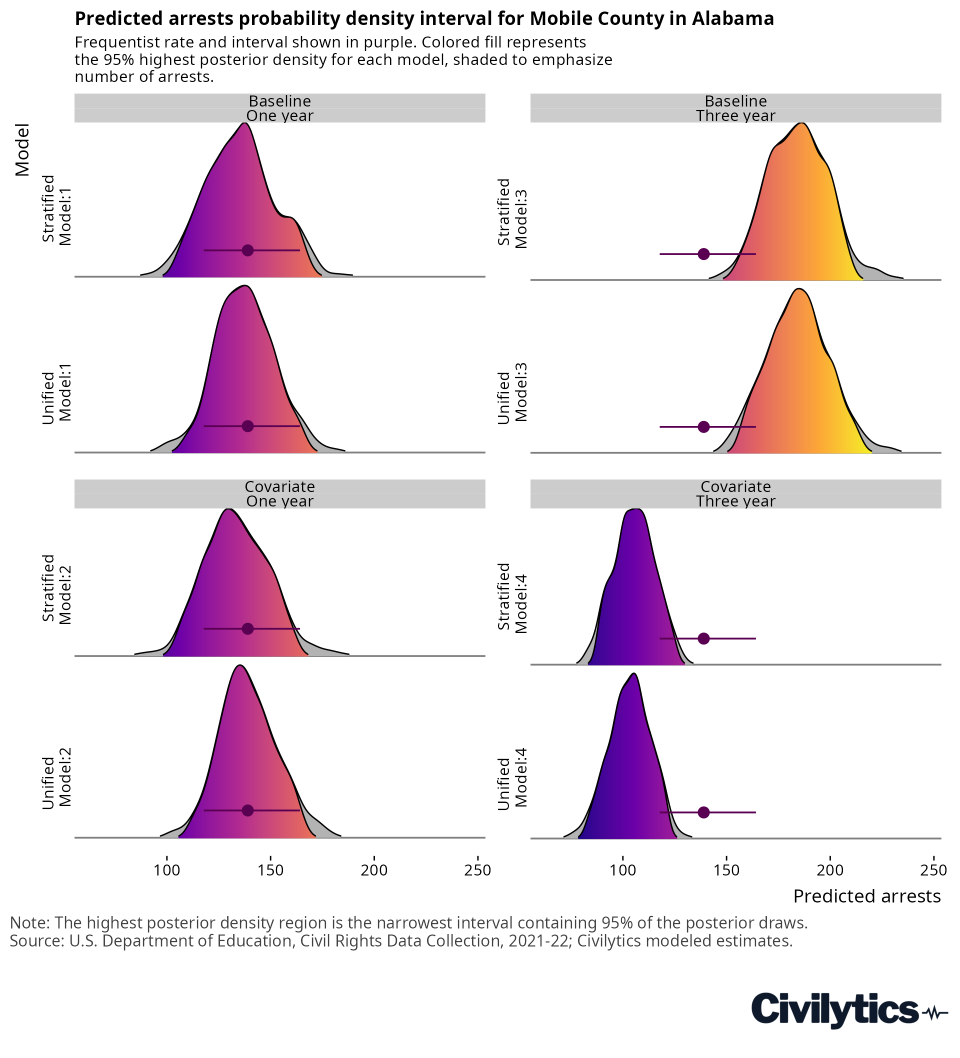
As we saw above, we can go beyond intervals and look at the distribution of likely arrests from the models. In the next figure, we plot the distribution of the draws from each model as density ridges with the 95% Bayesian highest posterior density (HPD) distribution represented in color and the full posterior distribution shown behind it in gray. The frequentist interval is represented as the black point interval. We see the one-year models on the left are all very similar, with the baseline models nearly perfectly recreating the frequentist interval and the stratified models having a wider tail. None of the three-year models align with the one-year models. The baseline models (top right) are shifted to the right (higher expected arrests), and the covariate models (bottom right) are shifted to the left (fewer expected arrests). In all cases, the HPD from the Bayesian models does still intersect with the frequentist interval.
A case study comparing differences
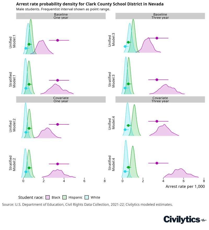
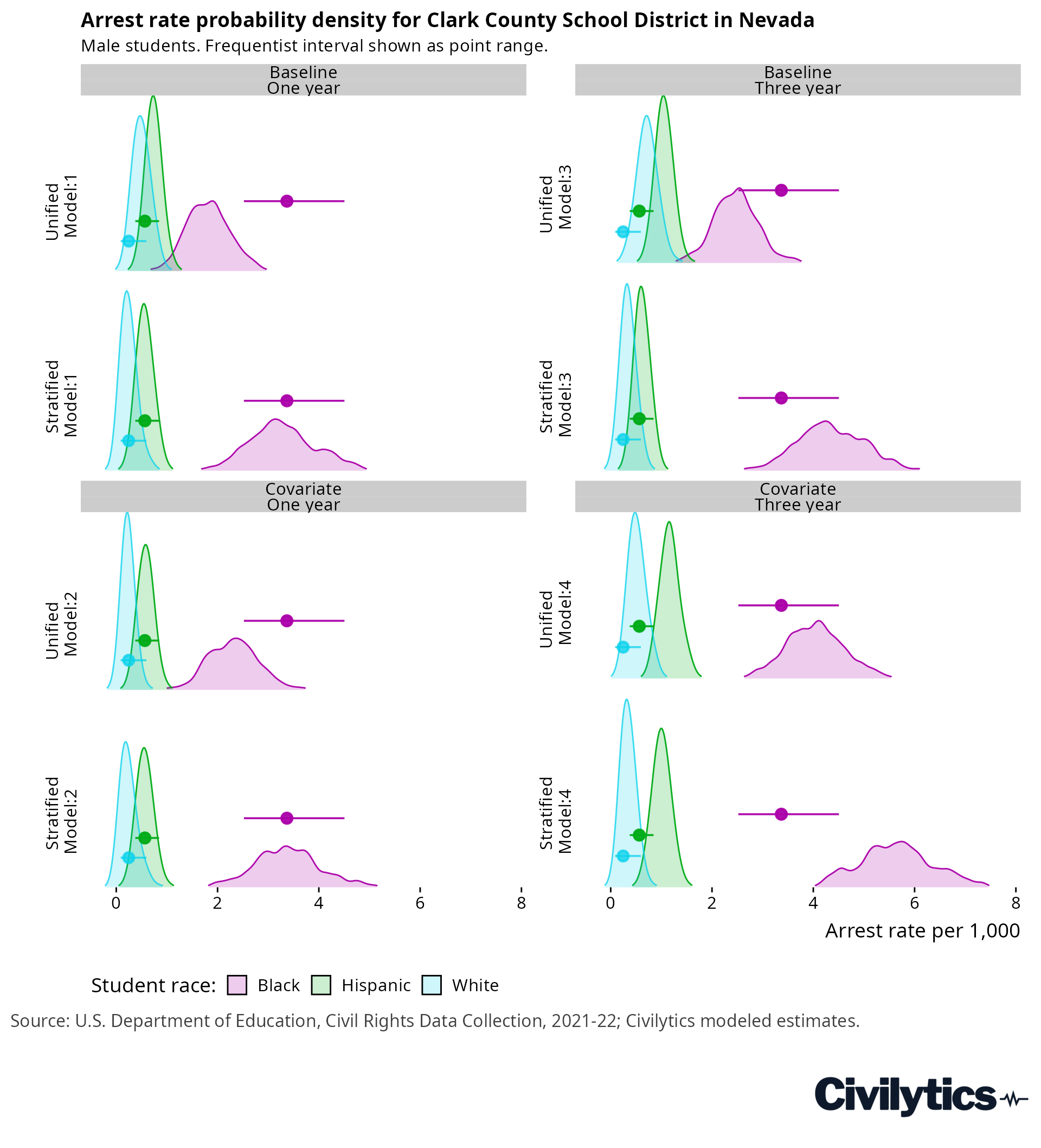
One of the major motivations for modeling arrest rates is to improve our ability to quantify demographic, geographic, and temporal differences in arrest rates in the face of the uncertainty posed by the sparse and rare nature of arrests. Below we take the case of Clark County, Nevada, where we model the arrest rates of three demographic groups: White, Hispanic, and Black male students. In the figure the Bayesian posterior density is plotted against the frequentist approximate interval (the point interval) for each group. The frequentist analysis (a comparison of the point intervals) allows us to confirm that Black male students have a notably higher arrest rate than Hispanic and White male students but does not allow us to distinguish between White and Hispanic students’ arrest rates (the intervals overlap).
In all cases, the Bayesian models agree that Black male students have a meaningfully different arrest rate than the other groups, though without covariates, unified models 1 and 3 predict the rate should be much lower than the frequentist estimate. In all cases, we observe substantial overlap in the distributions of Hispanic and White male students, though, in some cases like the covariate three-year models (bottom right panel), there is more distinction between the two distributions.
However, the difference in these intervals is not the same as the interval of the difference. With our Bayesian posterior samples, we can directly compute the distribution of the difference between White and Hispanic male students and plot that just like we have plotted the predicted values above. In the next figure we repeat the predicted arrest rates for White and Hispanic students in the top half of the figure, and, in the bottom half, plot the distribution of the model calculated difference between them. Even though the distributions have some overlap, particularly in the one-year models, when we calculate the difference directly, we see that all models predict a higher arrest rate for Hispanic students at least 84% of the time (Unified Model 1) and as much as 100% of the time (Stratified Model 4).
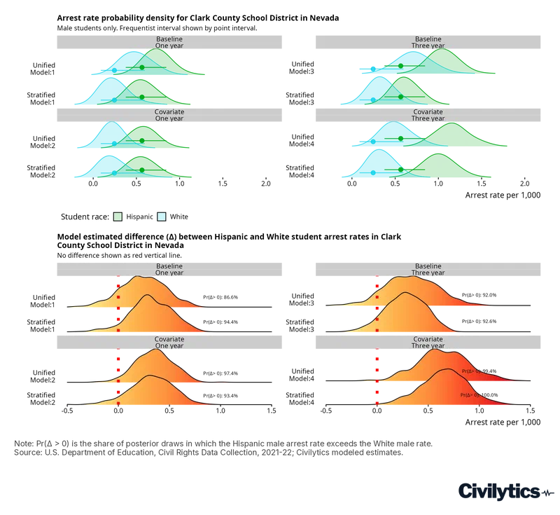
This example shows us the applied power of the Bayesian approach, which allows us to use draws from the posterior to calculate quantities of interest instantly as well as compute their probability in a straightforward way that allows us to answer questions using plain probability statements.
Comparing state-level demographic group differences
Finally, we return to Table 1, where we compared state arrest rates for selected demographic groups. We can now use the modeling approach to assess if there are differences for the selected demographic groups. As we discussed above, the frequentist intervals, shown in the top half of the figure as point ranges, are all overlapping due to the small sample sizes involved. For clarity we present two model specifications (one unified model, one stratified model). In the bottom panel, we present the distribution of the model predicted differences for two of the comparisons. In none of these cases do our models allow us to rule out the groups having the same rate – the sample size remains too small and the distributions too similar– but, depending on our use case, the information we do get can be useful. In the bottom left, there is up to an 80% probability that Colorado American Indian and Alaska Native students have a higher arrest rate than their Alaskan counterparts. In the bottom right, the two models do not agree whether Black or American Indian and Alaska Native students have higher arrest rates within Alaska – the stratified model predicts that Black students most likely have a higher arrest rate while the unified model predicts the opposite. In both cases, using statistical models allows us to examine these comparisons in more depth than either using the raw reported arrest counts or the frequentist arrest rate intervals.
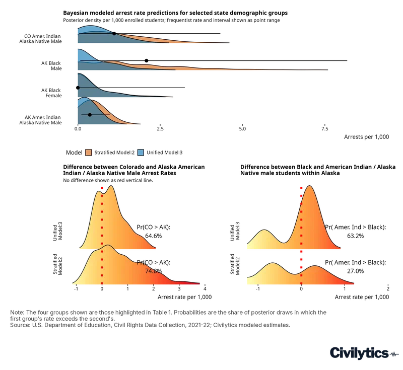
These examples are provided to illustrate how the investment in modeling sparse and rare events like arrest rates can make it easier to analyze and compare differences across geography, time, and demographic groups. By leveraging more information, we can increase the precision of our estimates, unlocking more potential comparisons, and by leveraging posterior-based inference to directly compute quantities of interest like group differences, we can construct a distribution of those differences and express them as probabilities. Using this approach can make it easier for more users of these data to confidently make probability assessments about differences between and changes in arrest rates.
Conclusion
We set out to understand if Bayesian hierarchical models could improve how researchers describe and measure a sparse and rare event like school-based arrests. Specifically, we sought to demonstrate the utility of applying these tools to demographic, geographic, and temporal comparisons among arrest rates. We found that in almost all cases Bayesian models improved upon a frequentist approach to describing arrest rates in three fundamental ways. First, Bayesian models almost always narrowed the arrest rate interval, and did so dramatically in the most common case of 0 reported arrests in small populations. This is not surprising as the frequentist interval in these cases, defined by the rule of three, is quite conservative. Still, this improvement is important because it increases precision not just the individual rates themselves but also of any aggregation of rates we create (such as calculating state-level student group arrest rates). Second, Bayesian models can incorporate covariates and/or multiple years of data to provide arrest rate estimates that further increase precision and smooth out reporting issues in the data. Much more work is needed to explore the tradeoffs associated with different combinations of prior years of data, covariates, and modeling assumptions – but the initial results show that providing options to users could improve comparison. Finally, using posterior prediction, the Bayesian approach provides data consumers with much greater flexibility in the types of comparisons they make and how they express and visualize those comparisons. By loading the posterior draws from the model into a database, users can write simple queries that correctly aggregate and combine the model predictions to construct quantities of interest and visualize them in compelling and clear ways.
Limitations
This study is a starting point and there are many important directions to continue to build tools that allow descriptive comparisons of arrest rates that are improved through statistical modeling. An important limitation here was the selection of our primary covariate of interest, referrals to law enforcement. Because this value was collected on the same form in the CRDC as our outcome of interest, it is likely that errors in reporting arrests are also highly correlated with reporting errors in referrals. Using this covariate kept our sample larger by not introducing missing data from other areas of CRDC, such as missing suspension data, but the high correlation with missing arrests made the covariate function more like an additional weight on the data in the current year and less like an independent measure. This limited the ability of our models to address suspicious underreporting in the arrest totals. An important next step could be to investigate if adding covariates collected outside of the arrests collection has a similar effect on coverage and precision, or if these covariates provide different information that results in different modeling properties.
Second, the models selected and fit here were chosen to balance computational feasibility with the realities of completing this study. There is likely substantial room to improve the coverage and precision of arrest rate estimates through a more thorough evaluation of various modeling strategies including perhaps additional geographic stratification, adjusting for nonlinearity based on sample size, or accounting for autoregressive trends in arrest rates over time with additional waves of data. We hope that the present study serves as a template for further exploration into the modeling space to better understand and make available a wider range of modeling options for making rigorous and precise demographic, geographic, and temporal comparisons in arrest rates.
Recommendations for future work
Bayesian posterior draws from a selection of model specifications should be made available to researchers to compare rare event rates like the arrest rates demonstrated here. With the release of each wave of the CRDC, these posteriors could be computed once and then made available as a dataset or web API for researchers to access within their statistical software of choice. This would eliminate the costly upfront steps of computation and allow researchers interested in describing and understanding arrest rate disparities easy access to more precise and easier to work with estimates. Meanwhile, work can continue on refining and extending the model specifications demonstrated here as well as communicating with prediction consumers about which model predictions to use to answer which questions. Collectively, this effort could extract tremendous additional value from the critically important Civil Rights Data Collection.
Appendix
Computation
The frequentist approach has one significant advantage over Bayesian modeling: it can be calculated instantaneously using standard statistical software. Calculating hundreds of thousands of approximate intervals can be achieved in less than a few seconds, even on very modest computer hardware. To access the advantages of the Bayesian models above, we must first estimate them.
To help guide future research applying models to sparse and rare events, we report the computation time, dataset size, and number of estimated parameters for our unified and stratified models below. We show how the time to fit models scales with the complexity of the model and the size of the dataset. For unified models we report the runtime to complete all four sampler chains; for the stratified models we report the sum of the runtime for the model fit to each of the eight subsets. We also report the number of parameters each model estimated. For unified models this includes the random intercepts and fixed effects. For the stratified models, it includes the sum of those parameters for each of the eight model subsets. Finally, some models required a longer sampling run – in terms of the number of iterations –to converge and provide stable results. In general, more complex models require a greater number of iterations to achieve convergence among the sampler chains and produce reliable estimates. We report the number of iterations per chain as it has a significant impact on runtime. Where necessary, more iterations were used to ensure that the sampling chains converged and that enough effective samples were obtained for analysis of the posterior.
| Models | Runtime in minutes | Data rows | Parameters | Iterations per chain |
|---|---|---|---|---|
| Unified 1 | 26.9 | 106703 | 16339 | 3,500 |
| Unified 2 | 62.6 | 106703 | 16340 | 3,500 |
| Unified 3 | 217.1 | 307468 | 17101 | 3,500 |
| Unified 4 | 375.4 | 307468 | 17102 | 4,000 |
| Unified 5 | 280.9 | 307468 | 17103 | 4,000 |
| Stratified 1 | 24.2 | 106703 | 107127 | 2,000 (x 8 models) |
| Stratified 2 | 48.3 | 106703 | 107135 | 3,500 (x 8 models) |
| Stratified 3 | 100.5 | 307468 | 120971 | 3,500 (x 8 models) |
| Stratified 4 | 117.3 | 307468 | 120979 | 4,300 (x 8 models) |
| Stratified 5 | 138.3 | 307468 | 120987 | 4,000 (x 8 models) |
Table 7: Model computation times
All models computed in R using the brms package to fit STAN models via the CMDSTANR interface. All models converged and showed no diagnostic issues with all parameter Rhat values being less than 1.01. Models were computed on a MacStudio M3 Ultra with 4 parallel chains with multithreading enabled at 4 threads per chain, requiring a total of 16 computer cores. Computing the multiyear models required a minimum of 64GB of RAM.19 Enabling within-chain threading improved performance for most models, though a full analysis of the best performing settings for the computational environment is outside of the scope of this work.
As we expect, adding rows of data does increase computation time: for unified models a 2.9x increase in rows led to a 5.6x increase in runtime; for stratified models the same runtime increases varied from 3.1x to 5.3x. As we expected, stratification is considerably faster (1.7-2.8x speedup), but stratified models have different predictive properties than the unified models: generally they improve precision less while having greater coverage. Stratified models also allow us to fit more parameters to evaluate within district student group disparities. Interestingly, adding predictors to the unified models did not have a meaningful impact on runtime, though it did impact the runtime of the stratified models.
After some failed attempts to fit all of the models, we realized great improvements in sampling efficiency by transforming the referral predictors to the log-scale and removing rows where the number of students enrolled was 0. We attempted to further improve performance by using OpenCL (Open Computing Language) to accelerate sampling with GPU acceleration. However, in our initial experiments on a more limited set of the data, we found OpenCL decreased performance and that the best performance was achieved through additional within-chain threading.
While the Bayesian approach requires substantial investment in computation, it can be done once and the results saved for instantaneous calculations using posterior draws to compute intervals of interest. As the CRDC is a biennial collection, researchers can compute the necessary models with each wave of data released and use the resulting estimates for analysis and study. That is the approach we took for this paper: storing 500 posterior draws from all 10 models for every observation in the data within a DuckDB on-disk database for analysis. The resulting database is 80GB in size.
Full details and access to the code used to process the data, fit the models, and generate the figures in this paper will be available at: https://www.github.com/civilytics/crdc-sae (opens in new tab)
References
Agresti, A., & Coull, B. A. (1998). Approximate Is Better than “Exact” for Interval Estimation of Binomial Proportions. The American Statistician, 52(2), 119–126. https://doi.org/10.2307/2685469 (opens in new tab)
Bacher-Hicks, A., Billings, S., & Deming, D. (2019). The School to Prison Pipeline: Long-Run Impacts of School Suspensions on Adult Crime (No. w26257; p. w26257). National Bureau of Economic Research. https://doi.org/10.3386/w26257 (opens in new tab)
Bacher-Hicks, Andrew, Stephen B. Billings, and David J. Deming. 2024. “The School-to-Prison Pipeline: Long-Run Impacts of School Suspensions on Adult Crime.” American Economic Journal: Economic Policy 16 (4): 165–93.
Bell, W. R., Basel, W. W., & Maples, J. J. (2016). An Overview of the U.S. Census Bureau’s Small Area Income and Poverty Estimates Program. In Analysis of Poverty Data by Small Area Estimation (pp. 349–378). John Wiley & Sons, Ltd. https://doi.org/10.1002/9781118814963.ch19
Brown, L. D., Cai, T. T., & DasGupta, A. (2001). Interval Estimation for a Binomial Proportion. Statistical Science, 16(2), 101–117.
Chung, Y., Gelman, A., Rabe-Hesketh, S., Liu, J., & Dorie, V. (2015). Weakly Informative Prior for Point Estimation of Covariance Matrices in Hierarchical Models. Journal of Educational and Behavioral Statistics, 40(2), 136–157. https://doi.org/10/gfgv9n (opens in new tab)
Darling-Hammond, S., & Ho, E. (2024). No Matter How You Slice It, Black Students Are Punished More: The Persistence and Pervasiveness of Discipline Disparities. AERA Open, 10, 23328584241293411. https://doi.org/10.1177/23328584241293411 (opens in new tab)
Davison, M., Penner, A., Penner, E., Pharris-Ciurej, N., Porter, S. R., Rose, E., Shem-Tov, Y., & Yoo, P. (2022). School Discipline and Racial Disparities in Early Adulthood. Educational Researcher (Washington, D.C.: 1972), 51(3), 231–234. https://doi.org/10.3102/0013189x211061732 (opens in new tab)
deBettencourt, L. U. (2002). Understanding the Differences between IDEA and Section 504. TEACHING Exceptional Children, 34(3), 16–23. https://doi.org/10.1177/004005990203400302 (opens in new tab)
Dixon, P. M., Ellison, A. M., & Gotelli, N. J. (2005). Improving the Precision of Estimates of the Frequency of Rare Events. Ecology, 86(5), 1114–1123. https://doi.org/10/dbs5c8 (opens in new tab)
Eypasch, E., Lefering, R., Kum, C. K., & Troidl, H. (1995). Probability of adverse events that have not yet occurred: A statistical reminder. BMJ: British Medical Journal, 311(7005), 619. https://doi.org/10.1136/bmj.311.7005.619 (opens in new tab)
Gelman, A., & Hill, J. (2006). Data Analysis Using Regression and Multilevel/Hierarchical Models. Cambridge University Press.
Gopalan, M., & Nelson, A. A. (2019). Understanding the Racial Discipline Gap in Schools. AERA Open, 5(2). https://eric.ed.gov/?id=EJ1220747 (opens in new tab)
Gottfredson, D. C., & DiPietro, S. M. (2011). School Size, Social Capital, and Student Victimization. Sociology of Education, 84(1), 69–89. https://doi.org/10/c97dh8 (opens in new tab)
Hanley, J. A., & Lippman-Hand, A. (1983). If Nothing Goes Wrong, Is Everything All Right?: Interpreting Zero Numerators. JAMA, 249(13), 1743–1745. https://doi.org/10.1001/jama.1983.03330370053031 (opens in new tab)
Homer, E., & Fisher, B. (2020). Police in schools and student arrest rates across the United States: Examining differences by race, ethnicity, and gender. Journal of School Violence, 19(3), 1–13. https://doi.org/10.1080/15388220.2019.1604377 (opens in new tab)
Knight, C., Grasha, K., & Horn, D. (2024, July 23). Data shows juvenile crime is down. Why do police and prosecutors say it’s getting worse? Cincinnati.Com | The Enquirer via Yahoo News. https://www.yahoo.com/news/data-shows-juvenile-crime-down-233021437.html (opens in new tab)
Li, W., Land, T., Zhang, Z., Keithly, L., & Kelsey, J. L. (2009). Small-Area Estimation and Prioritizing Communities for Tobacco Control Efforts in Massachusetts. American Journal of Public Health, 99(3), 470–479. https://doi.org/10/c6rrsr (opens in new tab)
Losen, D. J., & Martinez, P. (2020). Lost Opportunities: How Disparate School Discipline Continues to Drive Differences in the Opportunity to Learn (p. 112). Learning Policy Institute; Center for Civil Rights Remedies at the Civil Rights Project, UCLA.
Martin, S. L., Stohs, S. M., & Moore, J. E. (2015). Bayesian inference and assessment for rare-event bycatch in marine fisheries: A drift gillnet fishery case study. Ecological Applications, 25(2), 416–429. https://doi.org/10/f645q3 (opens in new tab)
McElreath, R. (2020). Statistical rethinking: A Bayesian course with examples in R and Stan (Second edition). Chapman & Hall/CRC.
Na, C., & Gottfredson, D. C. (2013). Police Officers in Schools: Effects on School Crime and the Processing of Offending Behaviors. Justice Quarterly, 30(4), 619–650. https://doi.org/10.1080/07418825.2011.615754 (opens in new tab)
National Equity Atlas. (n.d.). Policing in Schools. Retrieved September 29, 2025, from https://nationalequityatlas.org/indicators/Policing_schools (opens in new tab)
Perry, B. L., & Morris, E. W. (2014). Suspending Progress: Collateral Consequences of Exclusionary Punishment in Public Schools. American Sociological Review, 79(6), 1067–1087. https://doi.org/10.1177/0003122414556308 (opens in new tab)
Rao, J. N. K., & Molina, I. (2016). Empirical Bayes and Hierarchical Bayes Estimation of Poverty Measures for Small Areas. In Analysis of Poverty Data by Small Area Estimation (pp. 315–324). John Wiley & Sons, Ltd. https://doi.org/10.1002/9781118814963.ch17
Riddle, T., & Sinclair, S. (2019). Racial disparities in school-based disciplinary actions are associated with county-level rates of racial bias. Proceedings of the National Academy of Sciences, 116(17), 8255–8260. https://doi.org/10.1073/pnas.1808307116 (opens in new tab)
Rohrer, J. M., & Arel-Bundock, V. (2025). Models as Prediction Machines: How to Convert Confusing Coefficients into Clear Quantities. PsyArXiv. https://doi.org/10.31234/osf.io/g4s2a_v2 (opens in new tab)
Skiba, R. J., Arredondo, M. I., & Williams, N. T. (2014). More Than a Metaphor: The Contribution of Exclusionary Discipline to a School-to-Prison Pipeline. Equity & Excellence in Education, 47(4), 546–564. https://doi.org/10.1080/10665684.2014.958965 (opens in new tab)
Stephens, C. P. (2024, August 1). The False Narrative of a Youth Crime Surge: What Educators Should Know. Education Week. https://www.edweek.org/leadership/the-false-narrative-of-a-youth-crime-surge-what-educators-should-know/2024/08 (opens in new tab)
U. S. Government Accountability Office. (2024, July 8). K-12 Education: Differences in Student Arrest Rates Widen when Race, Gender, and Disability Status Overlap | U.S. GAO. https://www.gao.gov/products/gao-24-106294 (opens in new tab)
U.S. Census Bureau. (n.d.). Small Area Estimation. Census.Gov. Retrieved November 8, 2021, from https://www.census.gov/topics/research/stat-research/expertise/small-area-est.html (opens in new tab)
U.S. Department of Education. (2023). 2020-21 Civil Rights Data Collection A First Look: Students’ Access to Educational Opportunities in U.S. Public Schools. https://www.ed.gov/media/document/crdc-educational-opportunities-reportpdf-21412.pdf (opens in new tab)
Ward, G., Petersen, N., Kupchik, A., & Pratt, J. (2021). Historic Lynching and Corporal Punishment in Contemporary Southern Schools. Social Problems, 68(1), 41–62. https://doi.org/10/gncqc7 (opens in new tab)
Weisburst, E. K. (2019). Patrolling Public Schools: The Impact of Funding for School Police on Student Discipline and Long-term Education Outcomes. Journal of Policy Analysis and Management, 38(2), 338–365. https://doi.org/10.1002/pam.22116 (opens in new tab)
Welch, K., Lehmann, P. S., Chouhy, C., & Chiricos, T. (2022). Cumulative Racial and Ethnic Disparities Along the School-to-Prison Pipeline. Journal of Research in Crime and Delinquency, 59(5), 574–626. https://doi.org/10.1177/00224278211070501 (opens in new tab)
Welsh, R. O., Joseph, B., & Rodriguez, L. A. (2025). Examining the Differential Relationships Between School Climate and Students’ Disciplinary Outcomes: Evidence from New York City. Educational Policy, 08959048251340878. https://doi.org/10.1177/08959048251340878 (opens in new tab)
Whitaker, A., Torres-Guillen, S., Morton, M., Jordan, H., Coyle, S., Mann, A., & Sun, W.-L. (2019). Cops and no counselors: How the lack of school mental health staff is harming students. American Civil Liberties Union. https://www.aclu.org/sites/default/files/field_document/030419-acluschooldisciplinereport.pdf (opens in new tab)
Williams, J. A., & Wiley, K. E. (2025). A New School Discipline Fulcrum: Identifying and Rectifying. https://doi.org/10.26153/TSW/58402 (opens in new tab)
Wolf, K. C. (2013). Booking Students: An Analysis of School Arrests and Court Outcomes. Northwestern Journal of Law and Policy, 9(1), 58–87.
Yang, M., Khan, F. I., & Lye, L. (2013). Precursor-based hierarchical Bayesian approach for rare event frequency estimation: A case of oil spill accidents. Process Safety and Environmental Protection, 91(5), 333–342. https://doi.org/10/gn67rz (opens in new tab)
Zhang, Z., Zhang, L., Penman, A., & May, W. (2011). Using Small-Area Estimation Method to Calculate County-Level Prevalence of Obesity in Mississippi, 2007-2009. Preventing Chronic Disease, 8(4), A85.
The 2023-24 CRDC data collection was expected to be completed by summer 2025, with data released in 2026 (U.S. Department of Education n.d.) but there is concern that the data may not be prepared and released as planned (MCR News 2025). ↩︎
Because of the pandemic, the planned 2019-20 CRDC was postponed to 2020-21. Outcomes and student experiences as reflected in the 2020-21 CRDC were greatly influenced by the pandemic, including widespread use of virtual and hybrid instruction (U.S. Department of Education, 2023). In the 2020-21 CRDC, only about a quarter as many arrests (9,738) and referrals (65,312) were reported as in 2021-22 (authors’ calculations). Thus, we do not include the 2020-21 CRDC as a prior wave of data due to the large differences from other years. ↩︎
Of the 17,704 districts observed in 2021-22, 16,203 were also in the 2017-18 data, and, of those, 15,877 were also in the 2015-16 data. ↩︎
The other racial/ethnic categories reported in the CRDC are Asian, Hawaiian/Pacific Islander, and multiracial. As explained below, we focus particularly on arrest rates for White, Black, Hispanic, and American Indian students. Prior research has documented striking disparities in arrest rates for Black and American Indian students compared to White students (Darling-Hammond and Ho 2024; Homer and Fisher 2020; U.S. Government Accountability Office 2024). We included Hispanic students as well because of their large and growing share of the U.S. student population. ↩︎
Out of 1,398,531 such enrollment records in 2021-22, 26,391 (1.9%) were excluded. ↩︎
It is important to note, however, that prior research has demonstrated striking inequalities in arrest rates by disability status (U. S. Government Accountability Office, 2024; Whitaker et al., 2019). ↩︎
Students with a 504 plan refer to students under Section 504 of the Rehabilitation Act of 1973. 504 plans cover all mental or physical impairments not specified in the Individuals with Disabilities Education Act (IDEA) and a 504 plan is different than an IEP which is only for IDEA-eligible disabilities (deBettencourt 2002). ↩︎
As a result, totals using our dataset will differ from publicly reported totals. ↩︎
Of the nearly 5.5 million arrest record rows by school, disability status, race, and sex, 3.37% (185,172 rows) are recoded to 0. ↩︎
Out of 98,010 schools in the CRDC, 2,756 are excluded by this rule (2.8%). These schools had 443 arrests (1.2%) and 914,380 students (1.8%). ↩︎
This restriction excludes 19.78 million students (40.8%) but only 1,453 arrests (4.2%) in 2021-22. ↩︎
This filters out 308 districts with 4,693 students (<0.01%) but only 1 arrest. ↩︎
We prefer the Agresti–Coull approximation over other binomial proportion confidence interval approximations as it has been found to be suitable for cases where the number of trials is as low as 40, which is much of our sample (Brown et al., 2001). ↩︎
g() is the logistic link function in our generalized linear model. We omit it in notation from the remaining model specifications for clarity. We explored alternative link functions, such as Beta regression of the rate directly and zero-one inflated beta regression but ran into computational challenges in fitting the models to a dataset this large and this sparse. ↩︎
This greatly increases sampling speed, the time it takes to fit the models, and has minimal impact on the results given the volume of data, which allows the data estimates to quickly overwhelm the priors. ↩︎
In 21% of cases, there is no variance in the draws, in which case we apply the Agresti–Coull correction to the standard deviation, resulting in an identical standard deviation to the frequentist intervals – the models and the data are tied (equal). ↩︎
Out of 106,703 observations, 101,974 have no arrest observed (95.5%). Simply guessing 0 would provide better than 95% coverage. ↩︎
We calculate the arrest rate for the largest 100 districts, rather than simply the national average arrest rate because, as we saw above, the national rate is strongly biased toward 0. ↩︎
At the time of this writing, the cost to rent the computing required for these models (a 32-core CPU with 64GB of RAM) is between $1 and $1.50 per hour. Producing these estimates should cost between $1 and $8 per model once the data are prepared. ↩︎